
Quasicrystals
Do quasicrystals, the physics of the atomic nucleus, the zeros of the zeta function, crystalline measurements and the Fourier transform have anything in common? Well, a lot, as you will find out if you read on.
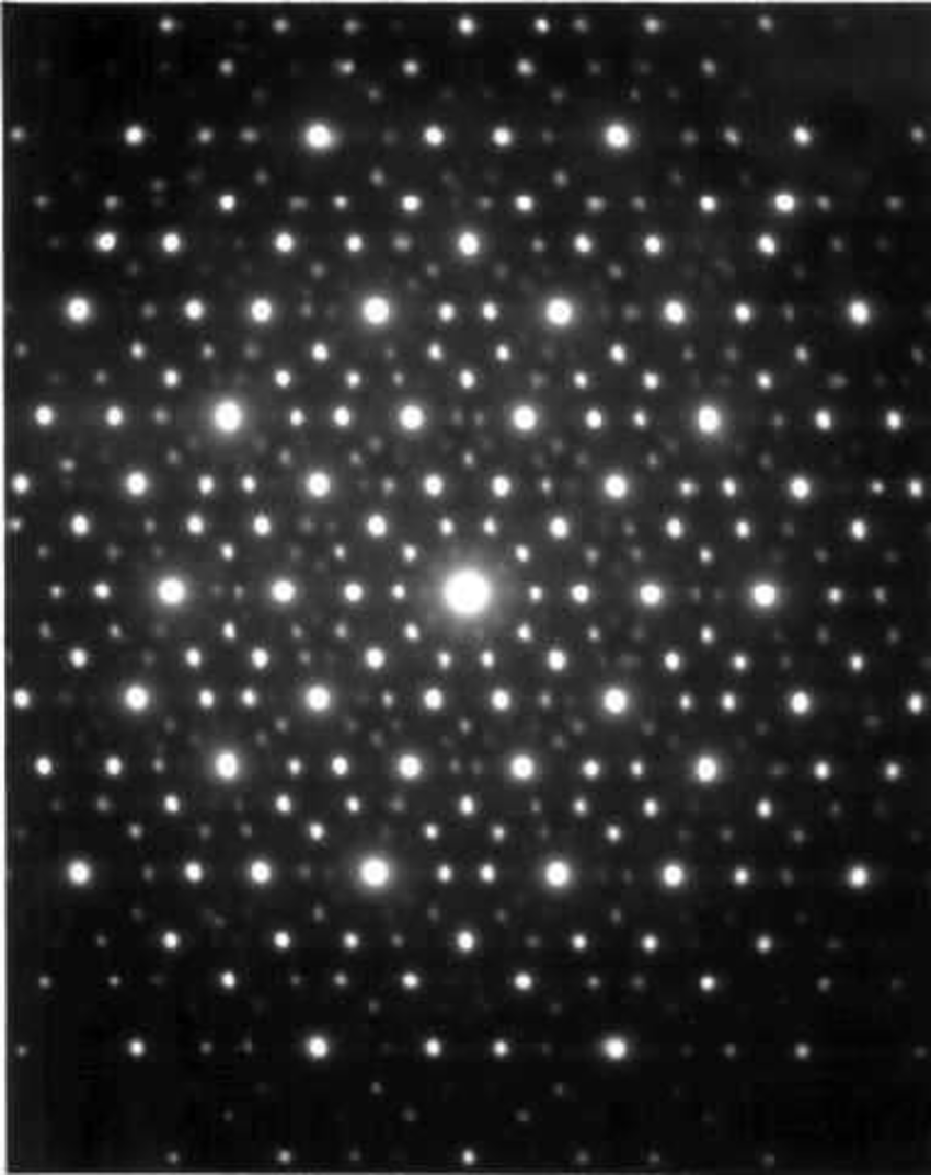
Dan Schechtman was awarded the Nobel Prize in Chemistry in 2011 for his discovery in 1984 of the quasicrystals. The delay was partly due to the hostility of Linus Pauling (Nobel Prize in Chemistry in 1954 and Nobel Peace Prize in 1962 and leader of the Chemical Society) who went so far as to say that there were no quasicrystals but quasi-scientists. The problem is that crystallography was a very mathematical science with its theorems forbidding pentagonal symmetries in crystals. Crystals consisted by definition of a set of atoms arranged in a repeating parallelepiped in space, each nucleus located at the points of a lattice. The following diffraction figure obtained from an aluminium-manganese alloy leaves no doubt about the pentagonal structure. This demonstrates the existence of ordered but non-periodic structures of atoms unlike those of classical crystallography.
Not a quasi-scientist, as Pauling said, but a quasi-president. Schechtman ran for president of Israel in the 2014 elections, getting only one vote in the final ballot. I wonder how many members did his family unit have?
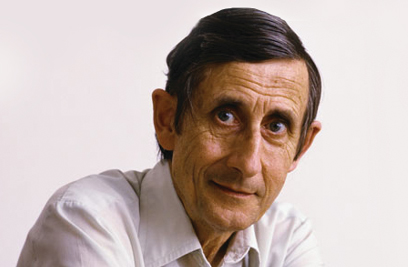
Freeman Dyson
A turning point in the study of the zeros of the zeta function was the meeting in 1973 between the young mathematician Hugh Montgomery (29) and the mature Freeman Dyson (50) at the Institute for Advanced Study in Princeton. Montgomery explained that he had studied the correlation of zeros of zeta and, before he presented his results, Dyson asked him if what he had found was the distribution $$1-\Bigl(\frac{\sin\pi x}{\pi x}\Bigr)^2.$$ “Exactly, how did you guess?” These are the correlations of the eigenvalues of the random Gaussian unitary matrices. These matrices were the model for the impossible-to-exactly-analyse Hamiltonians of nuclear physics. This comment by Dyson reinforced the earlier idea that the ordinates \(\gamma_n\) of the zeros of the zeta function are the eigenvalues of an operator in a certain space, which was a possible way to prove the Riemann hypothesis.
But besides the fact that this meeting served to introduce us to the heterodox Dyson, I would like to talk about one of his last activities (he died this February 2020). He was invited to give the American Mathematical Society’s AMS Einstein conference in 2008. Although he was unable to give it, it was published in the AMS Notices: Birds and Frogs.
Birds and Frogs
Dyson divides mathematicians into two classes: Birds and Frogs. Birds fly and look at the horizon, create theories and have great visions for the future of mathematics. Descartes unifying Algebra and Geometry or Grothendieck with his definition of schemes, the new spaces of Algebraic Geometry, are good examples of birds. Frogs like to splash around in the water and mud, where they can find flowers to contemplate or a stone that is rounder than the others. Ramanujan with his amazing formulas, or Robert Griess building the Monster group are good examples of frogs. But the most remarkable part of this lecture is when Dyson addresses the younger audience to propose a way to prove the Riemann hypothesis:
Quasicrystals exist in one-, two- or three-dimensional spaces. From a mathematical point of view, those of dimension 1 are of more interest. A crystal is a discrete distribution of point masses whose Fourier transform is a discrete point distribution of point frequencies. If the Riemann hypothesis is true, then the zeros of the zeta function form a one-dimensional quasicrystal and its Fourier transform is also a point distribution with masses in the logarithms of the primes and their powers. “My suggestion,” said Dyson, “to solve the Riemann hypothesis is to obtain a complete classification of the one-dimensional quasicrystals. A good task for frogs. Well, among them we will find the quasicrystal formed by the zeros of the zeta function and thus we will have proved the Riemann hypothesis”.
What we want to report here is just one important milestone of this programme which has just been completed last month.
Guinand
Andrew Guinand (1912-1987) was a student of Titchmarsh who, after a tour of Cambridge, Göttingen and Princeton, returned to his homeland, Australia, but finished his career in Canada. As a mathematician he is not well-known, but his name is always cited in connection with the explicit formulas of number theory. Recently, Meyer noted that his work contains the first examples of one-dimensional non-Poissonian quasicrystals.
Crystals are regular arrangements of atoms. When we treat them with sufficiently energetic waves each atom vibrates and we can see how on a screen the waves are superimposed and give us a diffraction figure consisting of luminous dots. We can say that we are looking at the Fourier transform of the dot distribution.
Classical crystals are explained by the fact that the Fourier transform of a set of unitary Dirac masses located at the points of a lattice has as its Fourier transform another distribution of point masses $$\mathcal{F}\Bigl(\sum_{a\in L} \delta_a\Bigr)=\frac{1}{\mathrm{vol}(C)}\sum_{b\in L’} \delta_b.$$ Or, in another way, if \(f\) and \(\widehat f\) are a function and its transform, fulfilling certain additional technical conditions, Poisson’s formula is satisfied, i.e. $$\sum_{a\in L}f(a)=\frac{1}{\mathrm{vol}(C)}\sum_{b\in L’}\widehat{f}(b),$$ with \(L\) being a lattice, \(L’\) its dual and \(C\) lthe unit cell of \(L\).
Changing his notation somewhat, Guinand proves that under certain conditions on the growth of \(f\) and its Fourier transform, we have $$\sum_{\gamma}f(\gamma)-f(i/2)-f(-i/2)=$$ $$-\frac{1}{2\pi}\sum_{n=1}^\infty\frac{\Lambda(n)}{\sqrt{n}}\Bigl\{\widehat{f}\Bigl(\frac{\log n}{2\pi}\Bigr)+\widehat{f}\Bigl(-\frac{\log n}{2\pi}\Bigr)\Bigr\}+\frac{1}{2\pi}\int_{-\infty}^\infty f(t)\Psi(t)\,dt,$$ with \(\Psi(t)\) being expressible in terms of the logarithmic derivative of the function \(\Gamma(x)\), and running \(\gamma\) through the ordinates of the zeros of the zeta function (we have assumed here the Riemann hypothesis). This is what Dyson has in mind when he says that the zeros form a quasicrystal. For the above expression essentially tells us that the transform of \(\sum\delta_\gamma\) is a sum of deltas at the points \(\pm\log n/2\pi\). But we see that here the situation is not as simple as in the Poisson formula.
The sum on the right hand side of the above equation is a sum in primes, although the coefficient \(\Lambda(n)\) somehow hides it. \(\Lambda(n)=0\) unless \(n\) is a prime or a power of prime \(n=p^k\) and in that case its value is \(\log p\). These coefficients are in fact the coefficients of the Dirichlet series development of the logarithmic derivative of \(\zeta(s)\) $$\frac{\zeta'(s)}{\zeta(s)}=-\sum_{n=1}^\infty\frac{\Lambda(n)}{n^s}=-\sum_p \sum_{k=1}^\infty \frac{\log p}{p^{ks}}.$$
Quasicrystals in Dimension 1
A paper has just been published resolving which are the quasicrystals of dimension 1.
Dyson is a physicist, you have to look at his proposal with an unfocused view, as if it were an impressionist painting. In the above expression, we see that the quasicrystal formed by the zeros is not entirely one-dimensional, it has two deltas located on the imaginary axis. Secondly, its transform is not exactly a sum of deltas, they are weighted deltas.
Dyson himself refers to the quasicrystals as a sum of deltas whose transform is a sum of deltas. There are many papers studying this problem in the general case of any dimension.
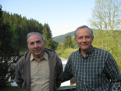
Two papers uploaded to arXiv this year, one in April by Pavel Kurasov and Peter Sarnak and the second in September by Alexander Olevskii and Alexander Ulanovskii have transformed the picture dramatically.
A crystalline measure is a sum of deltas $$\mu=\sum_{\lambda\in\Lambda} a_\lambda\delta_\lambda$$ whose Fourier transform has the same form $$\widehat{\mu}=\sum_{s\in S}b_s\delta_s,$$ with the sets of points \(\Lambda\) and \(S\) being discrete.
Both measures have to be tempered for the Fourier transform to make sense. If in addition the total variations are also tempered then \(\mu\) is said to be a Fourier quasicrystal.
The typical example arises from Poisson’s formula. A Fourier quasicrystal is of Dirac type if \(\Lambda\) is a finite combination of Poisson type quasicrystals.
What Kurasov and Sarnak do in their paper is to give a whole class of examples of non-Dirac type Fourier quasicrystals. Olevskii and Ulanovskii, looking at the examples, show that there are no others, that these are all the Fourier quasicrystals. But, to my mind, the most striking thing about Kurasov and Sarnak’s result is to see the examples and their properties. One would think that, since Kurasov and Sarnak have not found the zeros of the zeta function among their examples and since Olevskii and Ulanovskii have proved that there are no others, Dyson’s conjectures or intuitions were nothing but an old man’s dreams.
On the contrary, when I see the examples of Kurasov and Sarnak, I think that Dyson was absolutely right and very much on the right track in his conjectures. That now, more than ever, we should insist on following his suggestions. The frogs and the birds have to keep working. I will try to explain this in what follows.


Stable polynomials
Kurasov and Sarnak define a class of pairs of polynomials of several variables \(P(z_1,z_2,\dots, z_n)\), \(Q(z_1,z_2,\dots, z_n)\). A pair is stable if there exists a constant \(\eta\) and natural numbers \(\ell_j\) such that the functional equation $$Q(z_1,z_2,\dots, z_n)=\eta z_1^{\ell_1}\cdots z_n^{\ell_n}P(z_1^{-1},z_2^{-1},\dots, z_n^{-1}),$$ is verified and furthermore \(P\) does not have a zero at points with \(|z_k|<1\). There are many examples, but we are going to show only one that they put as the simplest, $$ P(z_1,z_2) =1-\frac13z_1+\frac13z_2^2-z_1z_2^2,$$ in which case \(Q=P\), \(\eta=-1\), \(\ell_1=1\) y \(\ell_2=2\). I leave to the reader the task of verifying the functional equation: $$P(z_1,z_2)=(-1)z_1z_2^2 P(1/z_1,1/z_2).$$
- Dyson’s first hit: The zeta function also verifies a functional equation.
The strategy of Kurasov and Sarnak is to construct from the polynomial a function \(F(s)\) and with its zeros the crystalline measure \(\mu\) will be constructed.
To construct \(F(s)\) from \(P\) we replace each variable \(z_j\) by \(b_j^{-s}\) where \(b_j>1\) is a number that we fix as we like. For example, I propose to take in the previous example \(b_1=2\) and \(b_2=\sqrt{3}\) and we obtain the function $$F(s)=1-\frac13\frac{1}{2^s}+\frac13\frac{1}{3^s}-\frac{1}{6^s}.$$ This function is a Dirichlet series.
- Dyson’s second hit: The zeta function is a Dirichlet series.
Since \(1/b_j^{-s}=b_j^{s}\), it follows that the functional equation of \(P(z_1,z_2)\) converts into a functional equation for \(F(s)\) $$F(s)=-\frac{1}{6^s}F(-s).$$ This is a particular case, but in general the zeros of \(F(s)\) lie on the imaginary line \(\Re s=0\).
- Dyson’s third hit: The (non-trivial) zeros of \(\zeta(s)\) lie on the critical line \(\Re s=\frac12\).
What do they prove? That if with the zeros \(i\gamma\) of our function \(F(s)\) we form the measure $$\mu=\sum_\gamma \delta_\gamma$$ we obtain a Fourier quasicrystal $$\widehat\mu=(\log 6)\delta_0-\sum_{n=1}^\infty \Lambda_F(n)(\delta_{\log n}+\delta_{-\log n})$$ where the coefficients are the figures that appear in the development $$\frac{F'(s)}{F(s)}=-\sum_{n=1}^\infty\frac{\Lambda_F(n)}{n^s}$$ and where \(\Lambda_F(n)=0\) unless \(n=2^a 3^b\).
- Dyson’s fourth hit: The crystal coefficients are those of the Dirichlet series of the logarithmic derivative.
We have cheated a little in choosing \(b_1\) and \(b_2\) as \(2\) and \(\sqrt{3}\), but with other choices it is not very different. I think the analogy with the zeta case is clear to anyone. But we can already notice that this example of Kurasov and Sarnak is a toy compared to that of the zeta function and the Riemann hypothesis.
The surprise in the paper by the Alexander’s, Olevskii and Ulanovskii, is that they prove that if a set \(\Lambda\subset\mathbf{R}\) is such that the sum of the deltas at the points of \(\Lambda\) is a Fourier quasicrystal, then it is one of those constructed by Kurasov and Sarnak from a pair of stable polynomials.
The X-ray of the Kurasov and Sarnak function is very similar to that of the zeta function, as we see in the picture below:
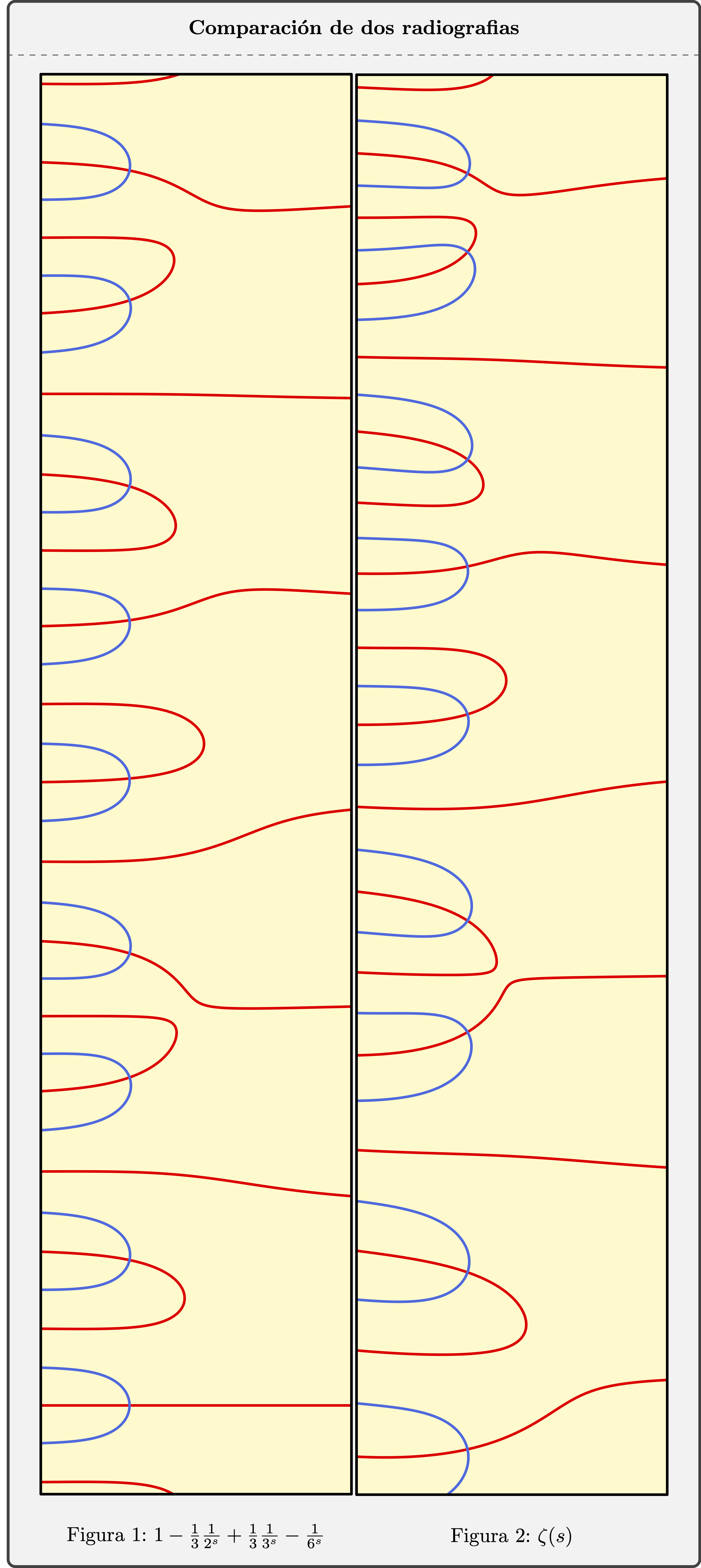
But the zeros of the \(F(s)\) function are spaced out, while those of the \(\zeta(s)\) function become more and more dense as \(\Im s\) increases. This difference is common to all the examples of Kurasov and Sarnak, as it is due to the fact that the functions are Dirichlet polynomials, while the series of \(\zeta(s)\) is infinite.
Learn more
Kurasov and Sarnak’s article has now been published and is freely available online. It can also be accessed via arXiv.
P. Kurasov, P. Sarnak, Stable polynomials and crystalline measures, J. Math. Phys. 61, 083501 (2020).
A surprisingly fast process, the authors submitted the paper on 29 April 2020, it was accepted on 10 July and published online on 3 August.
Olevskii and Ulanovskii’s paper was uploaded to arXiv very recently:
A. Olevskii, A. Ulanovskii, Fourier quasicrystals with unit masses, arXiv:2009.12810, 27 september 2020.
From my point of view it is much more technically complicated than the work of Kurasov and Sarnak. Kurasov and Sarnak are the Frogs, Olevskii and Ulanovskii are the Birds who have seen the whole picture.
Dyson’s lecture is also free on the net, it is an easy and entertaining read.
F. Dyson, Birds and Frogs, Notices Amer. Math. Soc. 56 (2009) 212–223.
This information would not be complete without mentioning Yves Meyer. He has contributed by studying and giving definitions of the mathematical point of view regarding quasicrystals even before they were found experimentally. His main book,
Yves Meyer, Algebraic numbers and harmonic analysis, Elsevier, New York, 1972,
has a sad history. The publisher Elsevier destroyed the existing copies in stock to make room in their warehouses. In 2018, when I had to consult the book, there was a used copy for sale on Amazon for 947.52 $.
In one of his papers, he gives examples of Fourier quasicrystals, prior to the papers we have been discussing.
Y. Meyer, Measures with locally finite support and spectrum, Proc. National Acad. Sciences, 113 (12) (2016) 3152-3158.
Hola, no me queda claro en este párrafo: “Lo que hacen Kurasov y Sarnak en su artículo es dar toda una clase de ejemplos de casicristales de Fourier que no son de tipo Dirac. Olevskii y Ulanovskii, viendo los ejemplos, demuestran que no hay otros, que esos son todos los casicristales de Fourier […] puesto que Kurasov y Sarnak no han encontrado los ceros de la función zeta entre sus ejemplos y que Olevskii y Ulanovskii han probado que no hay otros”, cuales son las implicaciones, ya que se da a entender primero que los casicristales tipo ceros de la función zeta no se han encontrado entre todos los ejemplos posibles y por tanto la idea no es factible y por otro se dice a continuación que sí merece la pena seguir buscando una solución de la hipótesis de Riemann en forma de casicristal con las propiedades de sus ceros.
¿Quizás cuando afirma que Ulanovskii y Olevskii han demostrado que no existen otros ejemplos que los de Sarnak y Kurasov se refiere solo a ejemplos de una clase que no incluye a los casicristales del tipo que darían los ceros de la función zeta?
Gracias
Ah, vale perdón. Releyéndolo he visto que efectivamente los ejemplos dados son de cristales que no son Dirac y el de la zeta es de tipo Dirac. Gracias de todos modos por la interesante entrada.
Los ceros de zeta no serían de tipo Dirac. Y Olevskii y Ulanovskii han probado que los encontrados por Kurasov y Sarnak son todos los que entran en la definición de casicristal que manejan. Pero los hechos parecen indicar que no están usando la definición adecuada.
Gracias, creo que entiendo ahora mejor la entrada. Quizás me podría comentar en qué medida está relacionada esta analogía de Dyson entre ceros de zeta en la línea crítica y casicristales o autovalores de ciertas matrices aleatorias, con la relación clásica entre zeta como L-función y la función Theta de Jacobi como forma modular que cumple la sumación de Poisson a través de una transformación regularizada de Mellin, o son conexiones totalmente independientes.