
In this post we will talk about boundaries: open and closed; fixed, free and mobile.
What is a boundary? According to the Cambridge Dictionary, a boundary is a real or imagined line that marks the edge or limit of something. We can also speak of an artificial boundary (whose line is drawn by the construction of artefacts or installations), an imaginary boundary (which follows a line fixed by means of astronomical or geometric references), a natural boundary (which follows and adapts to geographical accidents), etc.
In our world, boundaries play an essential role. They are often a real obstacle to equality and social justice. In an ideal world, one would be tempted to support open borders, so that human traffic would be subject to as few restrictions as possible. However, despite appearances, neither classical left-wing nor right-wing approaches have a definite position for or against open borders. Examples can be given: there are neoliberal currents that support unrestricted immigration, but there are also socialist currents that reject open border policies.
There are arguments for supporting and also to be against indiscriminate open borders: on the one hand, they are said to contribute to poverty reduction, a significant increase in global GDP and respect for human rights; on the other hand, it is argued that controlled borders encourage responsible policies in relation to population rates and that large-scale immigration from poorer to richer countries can create imbalances (for example, it is known that in 2010 there were more Ethiopian doctors in Chicago than in Ethiopia).
In science, we often talk about the frontiers of knowledge. Also, the frontier is sometimes identified with the boundary between two areas or disciplines. For example, an Operations Research specialist who solves problems with an important motivation in Finance ends up being labelled as a “frontier” in many cases. Something similar can happen to a numerical analyst interested in problems originating in (say) Quantum Mechanics. Unfortunately, the scientific community does not always look favourably on these situations, nor does it appreciate the added value of connecting two fields of work. Simply put, mathematicians tend to think that this activity does not correspond to priority objectives and, from the other side, an excess of mathematics is seen as something strange and even negative.
In Mathematics, the boundary has a very precise meaning: if \((X,\mathcal{T})\) is a topological space and \(Z \subset X\) is a given set, the boundary of \(Z\) is the set of points \(x \in X\) with the following property: every neighborhood of \(x\) cuts \(Z\) and its complementary. Thus, in the real line, the boundary of a bounded interval is the set formed by the extremes; in the plane, the boundary of a disc is the circumference that surrounds it and so on.
In the context of differential equations, boundary conditions are often referred to. They provide additional information to the equation: they tell (for example) which values takes the unknown at the boundary points.
Fixed boundary

An example that can help us to understand the role played by the boundary is that of a fluid occupying an approximately one-dimensional medium. Consider the particles of a gas moving inside a neon tube.
If we admit that the function \(u = u(x,t)\) determines the velocity of the particle at the point \(x\) at the instant \(t\), the tube occupies the spatial interval \([0,L]\) and the phenomenon develops along the interval \([0,T]\), it is reasonable to suppose that \(u\) is a solution of the Burgers equation.
$$
u_ t + u u_x – \nu u_{xx} = 0, \ \ (x,t) \in (0,L) \times (0,T),
$$
where \(\nu\) is a positive constant.
To identify the solution we are interested in, we must complement this equation with additional conditions. It is natural to fix the values of \(u\) for an initial \(t\):
$$
u(x,0) = u_0(x), \ \ x \in (0,L),
$$
where \(u_0\) (the initial particle velocity) is a known function. On the other hand, it is also natural to say something about the behaviour of \(u\) on the boundary of the interval \((0,L)\). For example, it makes sense to require that \(u\) verifies
$$
u(0,t) = 0, \ \ u(L,t) = 0, \ \ t \in (0,T),
$$
which means that, at the ends of the tube, the particles are at rest.
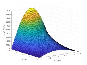
See Figure 2 for a visualisation of (a reliable numerical approximation of) the solution corresponding to \(L = 1\), \(T=20\), \(\nu = 0.01\) and \(u_0(x) = 0.05 \sin(\pi x)\).
Free border: a first example
Suppose now that the area of the tube occupied by the gas can change with time. More precisely, that the left end is fixed and the right end is mobile and ends up in a solid of mass \(m\) which is an obstacle to the expansion of the gas. Then, in principle, the gas particles move in an unknown domain. We find the equalities
$$
u_ t + u u_x – \nu u_{xx} = 0, \ \ x \in (0,\ell(t)), \ \ t \in (0,T),
$$
$$
u(x,0) = u_0(x), \ \ x \in (0,\ell(0)); \ \ \ell(0) = \ell_0, \ \ \ell'(0) = \ell_1,
$$
$$
u(0,t) = 0, \ \ u(\ell(t),t) = \ell'(t), \ \ t \in (0,T),
$$
to which must be added an additional equality relating the stress on the particles at the right-hand end and the acceleration of the solid:
$$
\nu u_x(\ell(t),t) = m \ell”(t), \ \ t \in (0,T).
$$
We are faced with a free boundary problem: the boundary of the region occupied by the gas particles. The data are \(T\), \(\nu\) and \(u_0 = u_0(x)\) (as before) and, in addition, the mass \(m\) and the initial position and velocity of the solid (\(\ell_0\) and \(\ell_1\)). Naturally, the numerical solution is far more complicated.
Other free boundary problems
Free boundary problems for differential equations (ordinary or partial differential) appear in a multitude of applications. They allow us to understand many phenomena that arise in physics, chemistry, biology, engineering, etc. We will now discuss three of them, today considered “classical problems”:
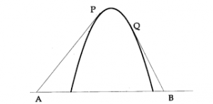
Obstacles – In its simplest version, the obstacle problem consists of finding the solution \(u = u(x)\) of
$$
– u_{xx} \geq f(x), \ \ u \geq \phi, \ \ – u_{xx} (u -\phi) = 0, \ \ x \in (0,L);
\ \ u(0) = u(L) = 0,
$$
where the functions \(f = f(x)\) y \(\phi = \phi(x)\) are given, with \(\phi(0), \phi(L) < 0\).
The solution is interpreted as the profile of a rope under time-constant stress that is held at the ends and cannot fall below an obstacle. The free boundary is the boundary of the region where \(u > \phi\); see Figure 3 for an illustration.
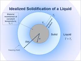
It makes perfect sense to consider similar problems in higher dimension (see Figure 4), with more complex differential operators, with time-dependent data and so on. Obstacle type problems have motivated and still motivate a lot of activity, lead to relevant and difficult questions and have many applications in physics and engineering; see for example [4,5,9].
Stefan-type problems – These are problems linked, among other phenomena, to the melting of ice; see Figure 5. The following simplified version (where \(k\) is a positive constant) is very similar to the formulation given in Section 2:
$$
u_ t – u_{xx} = 0, \ \ x \in (0,\ell(t)), \ \ t \in (0,T),
$$
$$
u(x,0) = u_0(x), \ \ x \in (0,\ell(0)); \ \ \ell(0) = \ell_0,
$$
$$
u(0,t) = u(\ell(t),t) = 0, \ \ t \in (0,T); \ \ u_x(\ell(t),t) = -k \ell'(t), \ \ t \in (0,T).
$$

Josef Stefan (1835-1893) was a Slovenian-Austrian physicist, mathematician and poet, student and later professor at the University of Vienna. He contributed to advances in physics in several directions: he discovered the law of power for black body radiation, studied heat conduction and diffusion in fluids, and helped to understand the problem that bears his name.
Stefan’s problems have been studied in depth for decades. For an account of relevant contributions, see [3,7].
Confined stationary vortices – In this case, we are dealing with a less familiar problem. It is to find a function \(u = u(x,y)\) defined on the rectangle \(\Pi = \{ (x,y) \in \mathbf{R}^2 : 0 < x < R, \ \ -S < y < S \}\) and a positive constant \(K\) such that
$$
-u_{xx} – u_{yy} = \lambda (u-Wx – K)_+, \ \ (x,y) \in \Pi,
$$
$$
u(x,y) = 0, \ \ (x,y) \in \partial\Pi \ \hbox{ (the boundary of \(\Pi\)),}
$$
$$
\int_\Pi |\nabla u|^2 \,dx\,dy = \eta,
$$
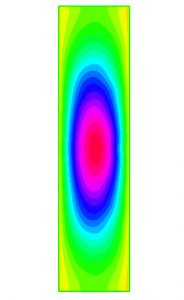
where \(\lambda\), \(W\) and \(\eta\) are given positive constants and \(z_+\) denotes the positive part of \(z\). The free boundary is the boundary of the region \(\Omega = \{ (x,y) \in \Pi : u(x,y) – Wx – K > 0 \}\). It is interpreted that \(\psi := u -Wx – K\) is the current function of a fluid that generates a flat vortex in \(\Omega\); see Figure 7 for a numerical solution, corresponding to certain values of \(\lambda\), \(W\) and \(\eta\). For more details on the problem, the interpretation of the solutions and their resolution, see [1].
Confinement often leads to models similar to the previous one. For example, the behaviour of plasma confined in a toroidal cavity (Tokamak machine) can be described by the solution of an analogous problem with the third identity changed by
$$
-\int_{\partial\Pi} \frac{\partial u}{\partial n} \,d\Gamma = I,
$$
where \(I\) is a new positive constant.
A very long list could be given, including (for example) problems originating in ecology (determining how the population of a species evolves in a habitat), social networks (calculating how fast a piece of news is transmitted to the collective), climatology (describing the advance of an avalanche or the spread of a tsunami), finance (valuation of financial assets), and so on. A collection of interesting problems can be found in [8].
Learn more
Free boundary problems have been studied by many researchers. Among them, we will mention here L. Caffarelli, A. Figalli, A. Friedman and J.L. Vázquez. The following references cover most of what is known, especially at the theoretical level. In particular, the reader will find in [10] an exhaustive analysis of the free boundary problems that arise in connection with the behaviour of fluids in porous media.
-
M.S. Berger, L.E. Fraenkel, Nonlinear desingularization in certain free-boundary problems. Comm. Math. Phys. 77 (1980), no. 2, 149-172.
-
L. Caffarelli, S. Salsa, Sandro, A geometric approach to free boundary problems. Graduate Studies in Mathematics, 68. American Mathematical Society, Providence, RI, 2005.
-
J. Crank, Free and moving boundary problems. The Clarendon Press,
 Oxford University Press, New York,1987.
 -
A. Figalli, Free boundary regularity in obstacle problems, arXiv:1807.01193v1 [math.AP].
-
A. Friedman, Variational principles and free-boundary problems, Second edition. Robert E. Krieger Publishing Co., Inc., Malabar, FL, 1988.
-
A. Friedman, Free boundary problems arising in biology, Discrete and Continuous Dynamical Systems, SERIES B Volume 23, Number 1, January 2018, pp. 193-202.
-
S.C. Gupta, The classical Stefan problem. Basic concepts, modelling and analysis. North-Holland Series in Applied Mathematics and Mechanics, 45. Elsevier Science B.V., Amsterdam, 2003.
- M.A. Piqueras, https://www.researchgate.net/profile/Miguel-Angel-Piqueras/publication/303959885_Problemas_de_frontera_libre_y_movil_algunas_aplicaciones_recientes_en_modelizacion_matematica/links/57601c6708ae2b8d20eb2566/Problemas-de-frontera-libre-y-movil-algunas-aplicaciones-recientes-en-modelizacion-matematica.pdf
-
X. Ros-Otón, Obstacle problems and free boundaries: an overview, SeMA Journal, volume 75, p. 399-419 (2018).
-
J.L. Vázquez, The porous medium equation. Mathematical theory. Oxford Mathematical Monographs. The Clarendon Press, Oxford University Press, Oxford, 2007.
Leave a Reply