
Traffic: catastrophes, inconveniences and models
It was perhaps the most notorious car crash in History. It took place on 30 September 1955 in Cholame (California, USA). On that day, James Dean, a 24-year-old actor who had become world famous with only three films, died.
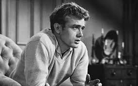
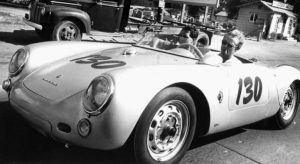
Dean was a big fan of speed. When he died, he was travelling to the town of Salinas, near San Francisco, to take part in a race in his car (a Porsche Spyder 550, nicknamed “Little Bastard”). However, it appears that he was not going very fast. In fact, the accident was not even his fault: a 23-year-old student driving a Ford Custom Tudor caused it when he missed a yield sign at an intersection on Route 466.
From time to time, traffic creates catastrophes. We all have in our minds dozens (maybe hundreds) of unfortunate accidents, sometimes due to the driver’s recklessness, but other times clearly unintentional and even unavoidable.
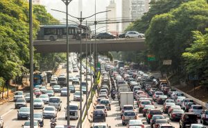
Traffic jams are another major transport problem. The root cause of a traffic jam is too many vehicles. For example, on a carriageway with two lanes in each direction, the maximum capacity is about 4,000 vehicles per hour. As the flow approaches this amount, vehicle speeds decrease, cars and trucks get closer and, when slowing down, the chances of a traffic jam increase dramatically.
I highly recommend the reader to read the article [1], which describes the five most famous (and disastrous) traffic jams in history. Two in particular are worth mentioning:
-
The one that took place in Sao Paulo (Brazil) on 23 May 2014, which reached the historical record of 344 km of accumulated traffic around the city.
-
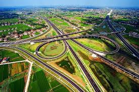
The one in China, on the G110 highway from Beijing to Tibet, “only” 100 km long, which lasted for … 11 days!
Mathematical techniques exist that allow traffic to be accurately modelled under multiple circumstances. See for example [2], where the authors present several predictive control proposals for traffic regulation incorporating variable speed limits in realistic situations. In particular, techniques of this type, adapted to the Grenoble ring road (France), lead to useful recommendations: the maximal speed at any given moment, the frequency of access, the use the reversible lanes, etc.
An equation for traffic
We will now consider a very simple situation (actually, the simplest among all possible scenarios), where we want to calculate the traffic density \(\rho = \rho(x,t)\) on a one-way road (say from left to right) occupying the points \(x\), with \(0 < x < L\), at time instants \(t\), with \(0 < t < T\).
The density \(\rho\) determines the traffic flow \(F\) and the traffic velocity \(V\). It is often assumed that
$$
F = V \rho – D \rho_x, \quad V = \frac{V_{\rm max}}{\rho_{\rm max}}\left(\rho_{\rm max} – \rho\right),
$$
where \(D > 0\) and \(V_{\rm max}\) and \(\rho_{\rm max}\) are maximal acceptable values for the velocity and density. Here and in the sequel, subscripts denote partial derivatives.
This all makes a lot of sense. On the one hand, the flux is a positive quantity, equal to the product of the velocity and the density, from which we must subtract another positive quantity, proportional to the spatial derivative of \(\rho\) (that is, to the variation of this function with respect to the variable \(x\); \(D \rho_x\) can be interpreted as a friction term). On the other hand, we say that the velocity is zero when the density reaches a maximum and grows linearly towards a maximum when \(\rho\) tends to zero.
Considering that, in any interval \(a < x < b\), the change in time of the density must coincide with the number of vehicles entering through \(x = a\) minus the number leaving through \(x = b\), it is easy to arrive at the equation that must be satisfied by \(\rho\):
$$
\rho_t + \left( \frac{V_{\rm max}}{\rho_{\rm max}}\left(\rho_{\rm max} – \rho\right) \rho \right)_x = D \rho_{xx} .
\quad\qquad\qquad\qquad\ \ \ \ (1)
$$
This equation is usually completed with information on the behaviour of \(\rho\) at the endpoints \(x = 0\) and \(x = L\) of the track and about the initial state of \(\rho\), i.e. its values for \(t = 0\):
$$
\begin{array}{c}
\rho(0,t) = u(t), \ \ \rho_x(L,t) = 0, \ \text{ for } \ 0 < t < T, \\
\rho(x,0) = \rho_0(x), \ \text{ for } \ 0 < x < L,
\end{array}
\qquad\qquad(2)
$$
The first mathematical task is therefore the following: given \(\rho_0\) and \(u\), calculate the solution of \((1)\)-\((2)\).
A numerical experiment
To solve \((1)\)-\((2)\), we have used a numerical method based on the following ideas:
-
First, the spatial derivatives are approximated by quotients in differences at a suitable set of points \(x_i\), with \(1 \leq i \leq m\). This allows the partial derivative equation \((1)\) to be replaced by an ordinary nonlinear differential system of dimension approximately equal to a reduced number of times \(m\).
-
A higher-order Runge-Kutta method is then used to solve the resulting system.
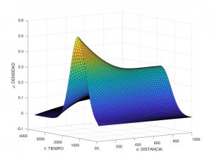
In Figure 5, we have visualised (a numerical approximation of) the solution of the preceding problem for
$$
\begin{array}{c}
L = 10^3~m, \quad T = 3.6 \times 10^3~s \ \ (10~h), \quad V_{\rm max} = L/T = 27.778~m/s \ \ (100~km/h), \\
\rho_{\rm max} = 0.555~veh/s \ \ (2000~veh/h), \quad D = 4 \times 10^4~m^2/s, \\
\rho_0(x) = 0, \quad u(t) = \rho_{\rm max} e^{-|t – T/5|^2/(2 \sigma^2)} \ \text{ with } \ \sigma = \sqrt{0.015}~s.
\end{array}
$$
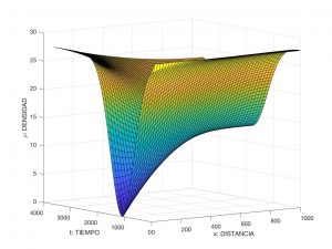
The velocity distribution is also presented in Figure 6.
Burgers’ equation
With simple variable substitutions, it is possible to rewrite \((1)\) in a much simpler way. Thus, by changing the variables \(x\), \(t\), \(\rho\) respectively by
$$
\tilde x := x/L, \quad \tilde t := t/T, \quad \tilde \rho := \rho/\rho_{\rm max}
$$
and denoting again \(x\), \(t\) and \(\rho\) the new variables, we arrive at a new equation
$$
\rho_t + \left(\left(1 – \rho\right) \rho \right)_x = \nu \rho_{xx} ,
$$
where \(\nu := D/(L V_{\rm max})\). Now, putting \(z := 2\rho -1\), we obtain for \(z\) the so-called Burgers’ equation (also known as the Bateman-Burgers equation):
$$
z_t + z z_x = \nu z_{xx} .
$$
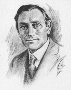
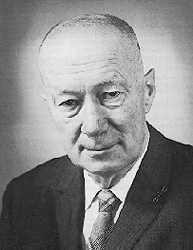
This equation actually appears in several areas of Applied Mathematics, related to fluid mechanics [3], nonlinear acoustics [4], gas dynamics, etc. It was introduced by the English mathematician Harry Bateman in 1915 (see [5]) and later studied by the Dutch physicist Johannes (Jan) Martinus Burgers in 1948 (see [6]).
Learn more
- See. The 5 most monumental traffic jams in history; James Dean’s car crash
- Domínguez Frejo, J.R.; Núñez Vicencio, A.; De~Schutter, B.; Fernández Camacho, E. – Hybrid model predictive control for freeway traffic using discrete speed limit signals, Transportation Research Part C, vol. 46, pp. 309-325, Sept. 2014.
- Landajuela, M. – Burgers equation, BCAM, 2011. Ver: https://www.bcamath.org/projects/NUMERIWAVES/Burgers_Equation_M_Landajuela.pdf.
- Hamilton, M.F.; Blackstock, D.T. – Nonlinear Acoustics, Academic Press, 1998.
- Bateman, H. – Some recent researches on the motion of fluids, Monthly Weather Review, 43(4), 163–170, 1915.
- Burgers, J. M. – A mathematical model illustrating the theory of turbulence, En “Advances in applied mechanics”, Vol. 1, pp. 171-199, Elsevier, 1948.
Leave a Reply