In this and the next post we will talk about inverse problems. We have already done so in several previous posts, for example here: Maths for not mistaking a tumour for a clot in a tennis player’s brain. We will give more information about the historical context, we will recall some of its countless applications and, in particular, we will talk about the famous Calderón problem, which has motivated (and still motivates) the work of many researchers.

Direct and inverse problems
For the sake of clarity, let us recall what it is to solve a general direct problem: we have a collection of data, we use them to carry out appropriate arguments and/or operations that produce certain results, and from these results we obtain useful information.
Thus, we can determine for example the trajectory \(x = x(t)\), \(y = y(t)\) of a particle in the plane knowing appropriate data: its initial position and velocity (\((x_0,y_0)\) and \((x_1,y_1)\) at time \(t=0\)), its mass (\(m\)) and the forces \(f = (f_x,f_y)\) acting on it. If we accept the postulates of classical mechanics, it will be enough to solve the differential system
where \(\ddot x\) and \(\ddot y\) denote the second derivatives respectively of \(x\) and \(y\). Once the trajectory is known, we can obtain (for example) the position of the particle at the instant \(t=1\) (the desired information).
Here, it is clear that the process allows us to determine the effect (the position at the final time) from the causes (the initial data, the mass and the forces).
In a reverse problem, the situation is more complicated and often more interesting: we know only part of the data and we also have access to the information (usually thanks to appropriate observations); and the task is to determine the other data.
In the example above, this question arises when, say, the initial velocity of the particle is unknown, but we know \(m\), \(f = (f_x,f_y)\), \((x_0,y_0)\) and, in addition, we are able to detect where the particle is for \(t=1\). We would be trying in this case to determine the causes from the effect.
In reality, in one way or another, we solve inverse problems every day. For example, in the morning, when we look out on the balcony, we are able to know whether it has rained or not in the preceding hours.
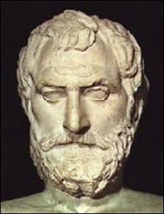
In mathematics, we can accept that the first inverse problem in history was solved by Thales of Miletus (around 640-546 BC): by measuring the lengths of the shadows of a staff and a pyramid cast by the sun, he easily deduced the height of the pyramid.

By the way, it is also told that one day, walking in the countryside, looking at the sky and meditating on the structure of the universe, he did not see a well in front of him and fell into it. A woman passing by laughed at him and asked him why he was so interested in knowing what was going on in the sky while neglecting what was right at his feet. This anecdote appeared in a Platonic dialogue; it was rewritten by Aesop and later by other storytellers, including Jean de La Fontaine.
It is well known that inverse problems are often ill-posed, i.e. either they do not have a solution for every choice of data, or the solution is not unique, or the solution does not depend continuously on the data.
History and applications
A historical example of an inverse problem is the discovery of Neptune from observed perturbations in the trajectory of Uranus.

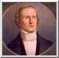
Planet Uranus was discovered in 1781 by Herschel. Between that year and 1847, having completed almost a full orbit, irregularities had been detected in its orbit that could not be explained unless the action of an additional planet was perturbing the trajectory. The plausibility of this hypothesis was demonstrated by the astronomers John Couch Adams (1819-1892) and Urbain Le Verrier (1811-1877) and confirmed shortly afterwards by direct observation. In fact, the discovery of Neptune led to the discovery of its moon Triton by Lassell only seventeen days later.
The mathematician François Arago, then director of the Paris Observatory, said that “Le Verrier had discovered Neptune with the tip of his pen”.
Interestingly, Le Verrier interpreted the anomaly in Mercury’s orbit (the well-known advance of its perihelion) as also being due to an undiscovered planet, which he called Vulcan. This generated a confusion that only ended in 1915, when Einstein put forward the General Theory of Relativity, which explained the phenomenon.
Significant examples of inverse problems are the following:
-
The determination of the distribution of mass from Newton’s law of gravity and observations made by gravimeters at different locations.
-
The distribution of magnetic properties of a medium from Maxwell’s equations and measurements of the magnetic field at different points using magnetometers.
-
The calculation of wave velocities and other geophysical characteristics using the wave equation and information provided by seismographs.
-
Also, the determination of the diffusion coefficients of a product, based on the usual diffusion equation (heat equation) and concentration values at different points.
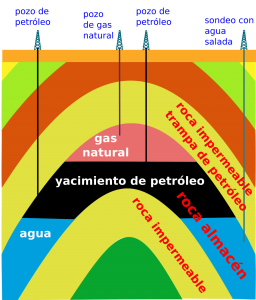
This gives an idea of the enormous number of applications related to inverse problems: they are frequently found in many areas of Physics (Mechanics, Thermodynamics, Electronics, etc.), in Engineering (for example in the context of oil exploration), in industry, in Medicine, …. They are also widely used in Meteorology, Oceanography, image processing, etc. See [1-3] for more details.
In recent times, machine learning and data assimilation techniques are being incorporated into the resolution of realistic inverse problems; see [4-5] for details.
Calderón

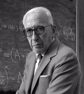
Alberto Calderón (1920-1998) is regarded as one of the most important mathematicians of the 20th century. He worked at the universities of Buenos Aires and Chicago. At the latter, together with Antoni Zygmund, he developed the theory that bears their names, concerning operators defined by singular integrals.
Calderón initially trained at the ETH (Eidgenössische Technische Hochschule) in Zurich and then at the University of Buenos Aires as an engineer. He was then hired by the state-owned oil company, YPF (Yacimientos Petrolíferos Fiscales), as a member of the research laboratory of the geophysics division. It was precisely there that he conceived the inverse problem that bears his name and which has motivated so much research to this day: place a medium in a region of the plane or space, and determine its electrical conductivity from measurements of the electrical potential and the current generated on the boundary (see the second part of this post for more details).
Some time later, having joined the University of Buenos Aires as a professor, he met Zygmund (then already a famous mathematician) during a visit of the latter. From that meeting arose a collaboration that would take him to Chicago and would keep him for more than thirty years producing results that would open up various lines of great interest. Among other contributions, let us mention the following: the Calderón-Zygmund Decomposition Lemma, invented to prove the weak type continuity of singular integrals of integrable functions; the uniqueness result of the Cauchy problem for equations in partial derivatives; the definition of the Calderón projector and the reduction of boundary problems for elliptic equations to singular integral equations on the boundary; the analysis of the Cauchy integral on Lipschitz-continuous curves, etc. See [6] for a significant selection of his work.
Learn more: initial velocity from the final position
Let us return to the inverse problem described in the first section. Suppose that the components \(f_x\) and \(f_y\) are given by
where (for example) \(4a_i m – b_i^2 > 0\) for \(i = 1,2\) and \((x_0,y_0) = (0,0)\).
It is then not difficult to reformulate the inverse problem as a linear system of 2 equations with 2 unknowns. Indeed, the solutions of the differential problem are given by
The only way we have to determine these constants is by imposing that the values of \(x(1)\) and \(y(1)\) are the desired ones: \((x(1),y(1)) = (x_d,y_d)\). But, unfortunately, for fixed \(x_d\) and \(y_d\), there do not always exist constants \(C_1\) and \(C_2\) with this property. For example, if we had \(4a_1 m – b_1^2 = 4 \pi m^2\) and we set \(x_d \not =0\), it would not be possible to find the constant \(C_1\).
Thus, we see that, in general, even when \(f_x\) and \(f_y\) are “simple” forces, determining the initial velocity of a particle travelling from the origin to a given point is not a well-posed problem.
For an introduction to inverse problems, I recommend reference [7], which corresponds to a course given by Otared Kavian several years ago at the University of Seville.
References
https://www.departement.math.uvsq.fr/pages-persos/kavian/ens

Leave a Reply