In a previous post How does a virus infect us? we briefly described the initial phase of an infection. Our aim in this entry is to present a simple mathematical model that is interesting enough from a biological point of view to show the subsequent evolution of the infection in our organism. Although the model we present is applicable, in principle, to any infection, we will focus on the current SARS-CoV2 coronavirus pandemic. In fact, the usefulness of mathematical models for decision-making during this pandemic has become clear. In just two months, different works have been developed, ranging from basic epidemiological modelling to estimate the infected population and mortality over time (in the context of COVID-19 see, for example, this interesting post), to more complex ones that have also indicated the peaks of saturation of hospital intensive care units in the autonomous regions of our country.
As a general rule, decision-makers and the media, as well as most citizens, focus primarily on the quantitative outputs of the models, such as the number of potentially infected and potentially dead people, which in turn is associated with the estimated availability of resources in the healthcare system. As can be deduced, alongside the specific quantitative results generated by the models is the estimation of the relative effects of possible interventions to help control and reduce the effects of CoVID-19 disease.
Clearly, the accuracy of model-derived estimates depends on the quality of the actual data available. Epidemiological data are, for example, the number of infections, deaths and tests performed, among others. In this sense, the variables to be included in the model will depend on the actual data against which the results will be compared, so it could be thought that simpler models may have a lower predictive capacity as they do not capture the real complexity of the disease. However, as Adam Kucharsky argues on social media, more complex models are not necessarily more effective than simple ones if key aspects of the biology are missed, so they can create a false illusion of realism and make it harder to detect possible omissions that are really important (in this respect see the interesting article by Ben Cooper on which Kucharsky’s claim is based).
Beyond, or before, epidemiological models, –and the social implications derived from them– are models that attempt to describe, also with rigorous mathematical language, the cellular processes underlying infection, which can be as simple or complex as we wish, depending on the number of variables to be included, the parameters that regulate them and the interactions that are established, all of this also depending on the real knowledge of their mechanisms and regulation and, of course, on the availability of actual data that can confirm their accuracy.
In this article, we present a model of viral infection that lies somewhere between popularisation and basic science, and which is neither simple nor complex. Specifically, we will model the first line of action of the immune system after the virus enters the body, the so-called innate immunity, which occurs before the second line of action, or adaptive immunity, takes place.
When we are infected by a virus, such as SARS-CoV-2 for example, as soon as the particle manages to enter a cell (for example a lung cell), a first line of response is activated based on a type of immune system cell called macrophages. In this case, the function of the macrophages is, on the one hand, to capture and eliminate the virus particles found in the environment and, on the other hand, to recognise and eliminate the cells (in the lung) infected by the virus. While this first defence is being carried out, macrophages emit signals that cause the immune system to prepare for a second line of response and thereby generate adaptive immunity, which involves other cell types, including antibody-producing lymphocytes. For more information, a simple and graphic explanation can be found in the recent article by África González.
Keeping all of the above in mind, modelling the first line of response should at least include how at this stage goes the variation of:
- the amount of virus, due to its multiplication when infecting cells or its decrease due to the effect of macrophages;
- the number of healthy cells susceptible to virus infection, which will increase by natural replenishment and decrease when infected; and
- the number of cells already infected, which may increase with infection and decrease if they die from viral overload or macrophage damage.
Given the recent emergence of CoVID-19, there are hardly any real data available to allow us to estimate the accuracy of the model for this particular disease. For this reason, we must point out that the parameter values we will use in the simulations are not real, but even so, they allow us to describe the dynamics of this mechanism, which forms part of the first line of action of the immune system.
Description of the model
To model the dynamics of the first line response after infection, we will consider the number of infectious particles (e.g. SARS-CoV-2 coronavirus) denoted by \(v\), the number of healthy cells susceptible to infection, \(x\), the number of cells that become infected, \(y\), and the number of macrophages involved, denoted by \(z\).
We could increase the complexity of the model by explicitly including other cell types, for example by quantifying the number of cells that recover after becoming infected, which only requires introducing the appropriate terms into the equations. However, in a first approximation, we will assume that virus-infected cells do not recover, i.e. the virus uses all its resources for replication when it enters the cells, after which the infected cells die. Or they are eliminated by the action of macrophages.
To try to describe the first line of immune system response to viral infection, we will use a combination of the models presented in [1, page 199]. Our main hypothesis will be that, once the virus enters the body (e.g. the lung in the case of SARS-CoV-2), the macrophages of the immune system act immediately by attacking the infective particles, but it still takes some time before they also start to eliminate the infected lung cells, which have stopped doing their original function because they are busy producing more viral particles.
Thus, in the present model, which is intended to simulate the first line of defence of the primary immune system, we will distinguish two phases: in the first phase, just as the first viral particles enter, the macrophages attack only the particles themselves, and in the second phase, the macrophages also attack the cells they recognise as infected.
First stage: the immune system eliminates only viral particles
As soon as a certain number of viruses enter the body, they try to penetrate cells in order to replicate. Just as they enter, the immune system’s first line of defence begins its work of eliminating the intruders, but for a while it may not recognise that there are infected cells, which it has to eliminate so that, if necessary, they can be replaced by functional ones.
Since the virus replicates in infected cells, we will assume, on the one hand, that the rate of replication is proportional to the number \(y\) of these cells, with a replication coefficient \(a\), and, on the other hand, that they die at a rate \(b\) due to the first action of the immune system. Thus, to model the dynamics of the virus population, we have the equation
\begin{equation}
(1)\qquad \qquad \frac{dv}{dt}=a y -b v.
\end{equation}
Let us now assume that healthy cells are constantly produced by the organism, at a rate \(c\), and that their natural death rate is proportional to their number, \(x\), with proportionality coefficient \(d\) which, for example, in the lung, is a very small value. On the other hand, such cells become infected on contact with the virus, with a rate that is proportional to the number of virus and the number of such cells (this is the typical term of a Lotka-Volterra predator-prey model see e.g. [1, page 54]). It follows from the above that the equation describing the dynamics of healthy cells is
\begin{equation}
(2) \qquad \qquad \frac{dx}{dt}=c-dx -\beta x v.
\end{equation}
Infected cells \(y\) die at a specific rate \(f\), which is the sum of the natural mortality rate \(d\) and the additional mortality rate due to viral infection \(e\) (i.e., \(f=e+d\)); their number increases proportionally to the product \(xv\) (which corresponds to the number of healthy cells that become infected),i.e.,
\begin{equation}
(3) \qquad \qquad \frac{dy}{dt}=\beta x v-(e+d)y.
\end{equation}
All parameters in equations (1), (2) and (3) are positive. In most cases it is also known that the coefficient \(d\) (the death rate of healthy cells) is much smaller than \(b\) (the disappearance rate of viral particles), so the quotient \(\epsilon=d/b\) is usually sufficiently small.
Thus, we obtain a system of three equations (1)-(3) governing the dynamics at the beginning of the infection, which must be solved with the initial conditions \(v(0)=v_0>0\), \(x(0)=x_0>0\) and \(y(0)=0\), since at the beginning it is assumed that there are no infected cells. Such a system is a non-linear system for which the total number of cells/virus is not constant, which differentiates this model from SIS or SIR models such as the one used in the above-mentioned entry. The reason for this is that the number of infectious particles could increase considerably without the number of healthy cells having to decrease in the same proportion, which is normal in a viral infection when the virus has a high replication capacity.
The system (1)-(3) has two stationary solutions
\begin{equation}(4) \qquad \qquad v_e=0,\quad x_e=\frac{c}d,\quad y_e=0,
\end{equation}
and
\begin{equation}(5)\qquad \qquad
v_e={{ac}\over{bf}}\left(1-\frac{1}{R_0}\right),\quad
x_e=\frac{c}{d}\frac{1}{R_0},\quad
y_e={{c}\over{f}}\left(1-\frac{1}{R_0}\right),
\end{equation}
where \(R_0\) is given by
\begin{equation}\label{R0}
(6)\qquad \qquad R_0=\frac{a\beta c}{bdf}.
\end{equation}
From the above it follows that for the virus to resist in the organism \(v_e>0\), which occurs only if \(R_0>1\). It is clear that the stationary solution (5) does not make biological sense if \(R_0<1\) because in that case the value of \(v_e\) would be negative (i.e. the virus is eliminated before reaching the value of the stationary solution). This quantity, \(R_0\) plays, at the cellular level, the same role as the well-known reproduction number that has been much talked about in recent times (for more information on the reproduction number in the context of an epidemic see this interesting article as well as [2]).
From the mathematical point of view it is interesting to mention that the solution (4) is unstable if \(R_0>1\) and stable if \(R_0<1\); that is, if the disease persists, then the solution (4) is unstable but, if it does not persist, then it is stable. Note that this result is consistent with cellular dynamics since, if after some time the immune system terminates the infection then, unlike solution (5), both the number of diseased cells and the number of viral particles must be zero.
In the present entry we will restrict ourselves to the case when \(R_0>1\), i.e. when in the first stage the infection persists and macrophages start to eliminate infected cells.
Second stage: the immune system eliminates both viral particles and infected cells
After a phase in which the immune system only attacks viral particles, macrophages also begin to eliminate diseased cells, as they represent a threat to organ function. To model this new action, we will modify equation (3) by subtracting the term \(\gamma y z\), corresponding to the interaction of the immune system (predator) with these diseased cells (prey), where \(z\) will denote the number of macrophages which, in turn, are produced at a constant rate \(g\) and die at a rate \(h z\).Thus, we will have the system of equations
\begin{equation}\label{eq-inm}(7)\qquad\qquad
\begin{cases}
\displaystyle\frac{dv}{dt}= & a y -b v \\[3mm]
\displaystyle\frac{dx}{dt}= & c-dx -\beta x v \\[3mm]
\displaystyle\frac{dy}{dt}= & \beta x v-(e+d)y-\gamma y z ,\\[3mm]
\displaystyle\frac{dz}{dt}= & g -h z ,
\end{cases}
\end{equation}
valid for \(t\geq\tau \). The initial conditions for the above system are nothing more than the values of the functions \(v(t)\), \(x(t)\) and \(y(t)\), solution of the system defined in (1)-(3) at the time instant \(t=\tau\), at which time the primary immune system starts to neutralise the diseased cells as well.
System (7) has two stationary solutions
\begin{equation}\label{sol-esi0}
(8)\qquad \qquad v_e=0,\quad x_e=\frac{c}d,\quad y_e=0,\quad z_e=\frac{g}{h},
\end{equation}
and
$$(9)\qquad
v_e={{ac}\over{bf}}\left(\frac{\alpha}{\alpha+\kappa}\right)\!\left(1-\frac{1}{R_0′}\right),\,
x_e= \frac{c}d\frac{1}{R_0′},$$
$$
y_e={{c}\over{f}}\left(\frac{\alpha}{\alpha+\kappa}\right)\!\left(1-\frac{1}{R_0′}\right),
$$
where
$$
\alpha=\frac{f}{d};\quad
\kappa=\frac{\gamma g}{dh}, \quad
R_0’=\frac{\alpha}{\alpha+\kappa} R_0,
$$
and \(R_0\) is the value above defined in (6).
From the analysis of the solution (9) it follows that, in this second stage, the infection will persist as long as \(R_0′>1\), since in this case \(v_e>0\). Conversely, if \(R_0′<1\), the immune system will eventually eliminate the infection since \(v_e<0\). Thus, for the immune system to eliminate the infection, the associated parameters (i.e., \(\gamma\), \(g\) and \(h\)) have to satisfy the following inequality
\begin{equation}\label{con-kill-vir}(10)\qquad \qquad
\kappa>\alpha(R_0-1)\quad\Rightarrow\quad \frac{g\gamma}{h}> f(R_0-1)=
{{a\,\beta\,c-b\,d\,f}\over{b\,d}}.
\end{equation}
In the latter case, it can be seen that the solution (8) is stable. This indicates that system (7) is suitable for modelling the performance of the primary immune system when it is able to neutralise the infection.
A numeric example
Let us now look at a numerical example that shows how the infection process occurs. We have taken the parameters so that \(R_0>1\). For this case we already know that the solution (5) is stable. The parameters corresponding to the immune system in the second stage will be taken in such a way that condition (10) is fulfilled, i.e. that our immune system is able to kill the infectious agent. In this case we know that the solution (8) is stable, i.e. after eliminating the virus the cells of the organism will recover after some time.
Take, for example, the following parameters
\begin{equation}\label{val}
a=1,\quad b=0.2,\quad c=1.75,\quad d=0.00175,\quad \beta=0.00005,\quad e=0.1\,
\end{equation}
in the system (1)-(3). For these values, \(R_0\approx 2.457>1\), and therefore infection prevails. With these parameters the solution (5) is stable.
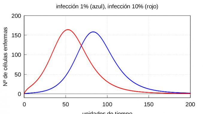
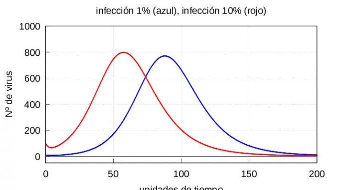
For the numerical resolution of the system (1)-(3) we will use two sets of initial conditions. In both cases we will take as initial value for the set of healthy cells the value \(x_0=c/d\) corresponding to the stationary value for equation (2) in case there was no infection. To differentiate a mild infection from a severe one, we will take as the initial value of \(v_0\) the values \(v_0=10\), corresponding to 1% of viral particles when compared to the number of healthy cells, and \(v_0=100\) corresponding to 10% of viral particles, respectively. That is, we will have the following two sets of initial conditions:
I: Mild exposure to the virus (1% viral particles) \(v_0=10\), \(x_0=1000\) and \(y_0=0\).
II: Severe exposure to virus (10% of viral particles) \(v_0=100\), \(x_0=1000\) and \(y_0=0\).
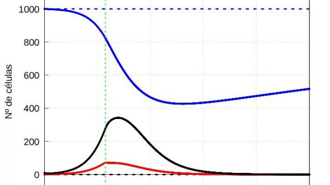
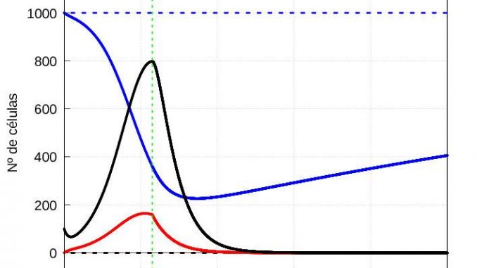
The results are shown in figures 1 and 2, respectively.
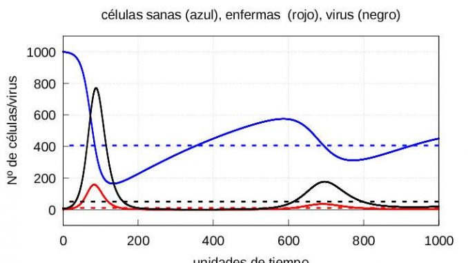
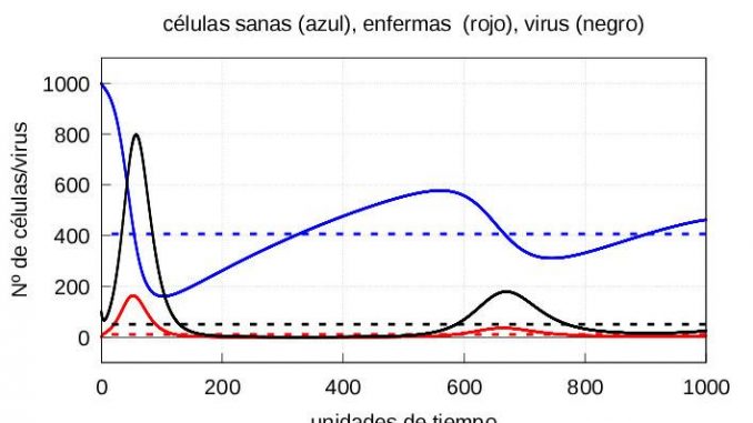
Note that in both cases, if we let the system (1)-(3) evolve for a sufficiently long time, the solution eventually converges to the stationary solution (5). On the other hand, if the number of viruses at the start is higher, then both the maximum number of infective particles \(v\) and the maximum number of diseased cells \(y\) are reached earlier, as shown in the graphs of the evolution of the infection in figures 3 and 4.
Let’s see what happens when the macrophages start attacking the diseased cells as well.
As we have already said, after a certain time \(\tau\) the macrophages start to eliminate the infected cells as well. For the sake of simplicity, we will assume that the time it takes for the macrophages to act on the infected cells is the same, regardless of the number of viral particles infecting the organism at the beginning. We are going to set the \(\tau\) value around the first maximum of the amount of virus for the case of a severe infection (see figure 4), which in our case is \(= 57.5\) time units.
We are interested in the fact that our organism recovers from the infection, so we will choose the parameters associated with the second stage of immune system action, \(g\), \(h\) and \(\gamma\), such that condition (10) is fulfilled so that we are guaranteed that the immune system eliminates the infection.
Thus, we will take the values
$$
g=0.05,\quad h=0.0025, \quad \gamma=0.0075,
$$
so that \(R_0=2.457\) and also
$$
\alpha=58.14,\quad \kappa=85.71,\quad \kappa-\alpha(R_0-1)=1>0.
$$
For the considered values, the solution (8) is stable and the solution of the system (7) will tend to the said stationary solution, which in our example is
$$
v_e=0,\quad x_e=1000,\quad y_e=0,\quad z_e=20.
$$
For the numerical resolution of the system (7), we will take as initial values those values we obtained at the time instant \(\tau=57.5\) for the cases of mild and severe infection discussed above, and as initial value of \(z(\tau)=10\). The corresponding graphs are depicted in figures 5 and 6, respectively.
The evolution of healthy cells (Figure 7) and diseased cells and viruses (Figure 8) should be shown separately:
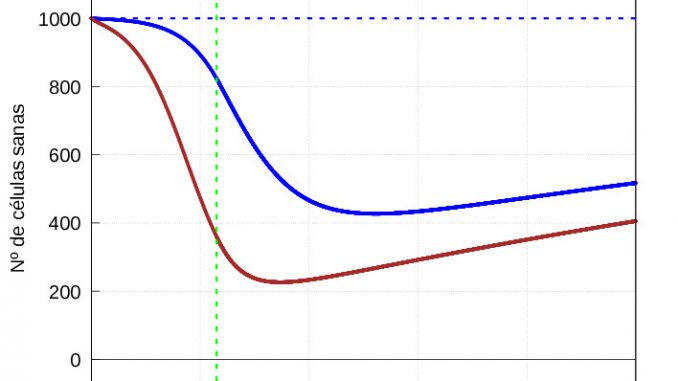
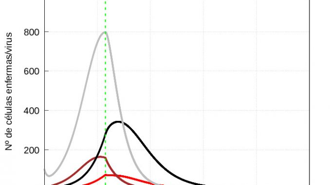
From figure 8, it is clear that when the immune system enters the second phase of action, it takes longer to kill the mild infection than the severe infection, i.e. when it starts to eliminate the infected cells, the immune system is much more aggressive in the case of a severe infection than in the case of a mild infection. However, because the damage done by the infection is much greater in the case of a severe infection, healthy cells take longer to recover than in the case of a mild infection (see figure 7). This is consistent with biology: the greater the damage, the longer they need to recover.
As a conclusion
The present study is an attempt to provide a qualitative insight into how the first line of the immune system responds to a viral infection, e.g. coronavirus, using a simple model that captures some of the main peculiarities of this biological process. The model is a predator (infective particles), prey (healthy lung cells) model. Unlike the SIR or SIS models, the total number of individuals (cells and virus) is not constant, which is justified by the fact that the number of infective particles could increase considerably without the number of healthy cells having to decrease in the same proportion (e.g. if you have a high replication rate for a virus).
Part of the simplicity of the model is to assume that cell dynamics are Malthusian and predator-prey. The main novelty is to assume that the primary immune system acts in two steps: first attacking only infectious particles and, after a certain time independent of the initial number of infected particles, also attacking diseased cells.
Despite its simplicity, there is no doubt that this mathematical model can be a good example of a dynamic system that, in a rigorous and interesting way, allows us to quantify the cellular response in our body, as occurs after infection by SARS-CoV-2, the pathogen responsible for CoVID-19.
References
[1] N.F. Britton, Essential Mathematical Biology, Springer, London, 2003.
[2] O. Diekmann, H. Heesterbeek, T. Britton, Mathematical Tools for Understanding Infectious Disease Dynamics, Princeton Series in Theoretical and Computational Biology, 2013, Princeton University Press.
You can download here this article in PDF format and the Maxima file with the calculations.

Leave a Reply