A simple example of mathematical modelling: The growth of populations

In a previous post we discussed the importance of the scientific method described by Galileo in his book Il Saggiatore. There we saw that in order to “understand” the world around us we need to use a combination of experience (performing experiments) and mathematics (mathematical modelling). It is this second part that we are going to deal with in this entry: mathematical modelling. Let us recall that the first phase of the scientific method consists of formulating, from the observations of certain phenomena, the mathematical equations to describe them. These equations, in a second phase, should allow us to predict the results of future observations, otherwise they should be discarded or modified by others that do. How to find these equations? That is exactly what mathematical modelling is about: finding the right equations to describe the phenomena in question. In this way, modelling consists of the following steps:

1. Quantifying the phenomenon, i.e. somehow converting the observations we make into quantities (numbers). This can be very “simple” (for example if we are interested in measuring velocities we can measure distances and times) but it can be very “complicated” (for example measuring the magnitude of a volcano eruption, something we will talk about in a future entry).
2. Postulate the equations that relate the magnitudes, in other words, find the set of mathematical formulae that relate them. Here, both the scientist’s intuition and luck play a fundamental role (an example that deserves a separate entry is how Schrödinger discovered the equation that today bears his name).
3. Compare the results obtained from the mathematical equations in step 2 with the observations made in step 1 and make further observations that may confirm the model. If they do not confirm the model, try to modify it accordingly and repeat the comparison.

For the sake of simplicity we will show how modelling works with a very simple to understand example: the growth of a population. Let’s imagine that we want to know how a population grows. One of the simplest models corresponds to the Malthus model already discussed in this blog and which was proposed by the English economist Thomas Maltus in 1798 in his famous “An Essay on the Principle of Population” (for further detail see this post). In it Malthus, based on data on the population of the United States in the 18th century, postulates that human population growth is exponential. Mathematically what this means is that the rate of population growth is proportional to the population, i.e. \(p'(t) = r p(t)\), where \(p(t)\) is the number of individuals in the population at time \(t\) and \(r\) is a certain constant (known as the population growth rate) that we must derive from the experimental data and \(p'(t)\) is the derivative of \(p(t)\) (which gives precisely the rate of growth). The solution of the above equation (which is a differential equation) is \(p(t)=p_0 e^{r(t-t_0)}\) where \(p_0\) is the number of individuals at the initial time \(t=t_0\). It is clear that if \(r<0\) the species will be condemned to extinction (see figure on the left) while if \(r>0\) we will have an exponential growth (see figure on the right) which, as commented in that post, is not realistic.

And it is unrealistic, among other things because if the number of individuals in the population increases too much, they will be forced to fight for space and resources, both of which are finite. Malthus estimated that food production grew in arithmetic progression (i.e. proportional to the number of individuals) while the human population grew exponentially, so he concluded that human beings were predestined to subsist in hunger and poverty. Although Malthus’ analysis turned out to be incorrect, it had a tremendous influence on his time. In fact it was his reading of Malthus’ essay in October 1838 during his trip around the world that induced Darwin’s now universally accepted mechanism of natural selection.

How can we correct the Malthusian model so that its predictions are more in line with experience? First of all, we must bear in mind that in the short term and under optimal conditions of space and resources (such as those in North America in the 18th century) the Malthusian model works quite well, and it is only when the number of individuals is very large that it begins to fail. On the other hand, it is well known that if the number of individuals grows, it tends to stabilise around a certain critical value. So the new model has to somehow predict for small populations an exponential growth and when the population is very large, a stabilisation of the population. The solution to the problem came from the Belgian mathematician and biologist P. F. Verhulst who in 1837 proposed the model known as the logistic model. His idea consisted of subtracting the term \(cp^2\) from the \(r p\) of the Malthus equation. Thus the new equation would be

\(p'(t)=r\,p(t)-c p^2(t),\qquad p(t_0)=p_0,\quad r,c>0. \)

Generally \(c\) has to be much smaller than \(r\) so that if \(p\) is not very large the Malthus equation is a fairly good approximation, but if \(p\) starts to grow too large then the \(-c p^2\) term becomes larger and ends up slowing exponential growth. Usually \(c\) is written as the quotient \(r/K\) where \(K\) is known as the carrying capacity of the medium and is a constant that is linked to the habitat resources. The solution of the Verhulst equation is

\(p(t)=\displaystyle \frac{r\, p_0}{c\,p_0 +(r-c\,p_0)e^{-r\,(t-t_0)}}, \)

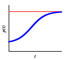
from which we can verify that for times close to the initial time \(t_0\) and for small values of \(p_0\), \(p(t) \approx p_0 e^{r(t-t_0)}\), that is, the exponential Malthus solution, is recovered. On the other hand, if \(t\) is very large (much larger than \(t_0\)), then \(p(t)\approx r/c=K\), i.e. the population stabilises. The behaviour of the population according to the logistic model can be seen in the following figure:

Let us now use the data compiled by the US Census Bureau on world population to estimate the parameters of the Verhulst equation and deduce what might happen to it in the not too distant future. If we use the data collected from 1950 (in that year the number of people was estimated to be \(2.558\cdot 10^9\)) until 2014, we obtain for \(r\) the value \(r=0.01731313844533347\). Thus, comparing the value given by Malthus’ formula \(p(2000)\approx 6.07837532775273232\cdot 10^9\) we see that it is quite similar to the real estimated value of \(6.088571383 \cdot 10^9\) people. On the other hand, the prediction for the year 2010 gives \(p(2010)= 7.22732389676767\cdot 10^9\) which starts to move away from the census estimate of \(6.866332358 10^9\). If we now use the logistic model keeping for \(r\) the same value as before and taking for \(c\) the value \(8.361178966147587\cdot 10^{-14}\) (which is obtained from the census data) we can use the Verhulst function to estimate the world population values. Thus, in 2010 the logistic model predicts a population of \(7.067929710275726 \cdot 10^9\), which is somewhat better (but not much) than that predicted by the Malthusian model (see figure).

What is interesting is to see that as we move away in time, the logistic model predicts the stabilisation of the population at a value close to \(2\cdot 10^{11}\), an amount that would be reached in the year 2200 approximately. The result is shown in the following graph.

In conclusion, the logistic model is still very simple because it does not take into account epidemics, wars, earthquakes or other disasters that unfortunately continue to occur in the world we live in. If we want to take such situations into account, we have to include new terms in the equation, terms that are generally not easy to understand. Surely, dear reader, by searching you can find several models that try to take this other situations into account, and if not, you can always try on by your own.