If the Riemann hypothesis is true, it will be by a hair’s breadth

How the zeros of the Riemann zeta function are arranged seems like the devil’s work. An unpublished paper by Brad Rodgers and Terence Tao shows us this for the umpteenth time. We can summarise their work by saying that if the Riemann hypothesis is true, it will be by a hair’s breadth.

Preliminaries on the zeta function

The zeta function is defined for \(\text{Re}(s)>1\) by means of the Dirichlet series $$\zeta(s)=\sum_{n=1}^\infty \frac{1}{n^s}.$$ Its connection with the primes comes at least from Euler who used it to give an analytic proof of the infinitude of the primes. But it was Riemann who studied it in depth. Riemann proved that it extends as a meromorphic function to the whole plane with a single pole at \(s=1\). The function \(\zeta(s)\) cancels out at negative even numbers. Apart from these it has infinitely many more mysterious zeros in the critical strip (\(0<\text{Re} (s)<1\)). Riemann conjectured that these zeros were all located on the straight line \(\text{Re}(s)=\frac12\). This hypothesis has not been proved to this day and is known as the Riemann Hypothesis (for brevity we will write RH in what follows).

These zeros are involved in the explicit formulae that express exactly sums depending on the  primes, such as \(\pi(x)\), the number of primes less than or equal to the positive real number \(x\).

To study the zeros Riemann constructed the function \(\Xi(z)\) defined by $$\Xi(z):=\frac{s(s-1)}{2}\pi^{-s/2}\Gamma(s/2)\zeta(s), \qquad \text{where \(s=\frac12+iz\)},$$ and \(\Gamma(s)\) is Euler’s Gamma function.

The function \(\Xi(z)\) is entire and has one zero for each zero of \(\zeta(s)\) in the critical strip and these are its only zeros. Thus the zeros \(\frac12+i\gamma\) of \(\zeta(s)\) on the critical line become the real zeros of the new function \(\Xi(\gamma)=0\). The RH is equivalent to the zeros of this function being all real.

Moreover the function \(\Xi(t)\) because of the normalising factor \(\pi^{s/2}\Gamma(s/2)\) is real on the real axis. The function \(\Xi(t)\) for real \(t\) tends to zero very quickly. That is why Riemann and all those who have subsequently calculated the zeros of \(\zeta(s)\) have used the function \(Z(t)\).

There are two real analytic functions with real values \(\vartheta(t)\) and \(Z(t)\) such that $$\zeta(1/2+it)=e^{-i\vartheta(t)}Z(t).$$ Since \(Z(t)\) is real its zeros can be detected as sign changes. And each real zero of \(Z(t)\) corresponds to a zero of \(\zeta(s)\) right on the critical line.

Precisely all the techniques for seeing that the zeros of \(\zeta(s)\) are on the line \(\frac12+it\) are based on detecting sign changes in \(Z(t)\). It is known that if \(Z(t)\) has a positive relative minimum or a negative relative maximum, then RH is false.

The Bruijn-Newman constant

Riemann wrote the function \(\Xi(t)\) as a Fourier transform. His result can be written by saying that
$$\frac18\Xi(t/2)=\int_0^\infty \Phi(u)\cos(tu)\,du$$ where $$\Phi(u)=\sum_{n=1}^\infty (2\pi^2n^4e^{9u}-3\pi n^2e^{5u})\exp(-\pi n^2e^{4u}).$$ This function is even \(\Phi(u)=\Phi(-u)\), but the formula does not tell us this. We have to use the properties of the modular forms involved in the construction of \(\Phi(u)\). We also see that \(\Phi(u)\) decreases super-exponentially to zero. Thus the Riemann hypothesis is transformed into proving that the zeros of the Fourier transform of \(\Phi(u)\) are all  real.

Newman in 1976, building on earlier work by de Bruijn, considers the function $$H_t(z):=\int_0^\infty e^{tu^2}\Phi(u)\cos(zu)\,du.$$ Since \(H_0(x)=\Xi(x/2)/8\), RH means that all zeros of \(H_0(x)\) are real.

In 1950 de Bruijn proved that all the zeros of \(H_t(x)\)  are real for \(t\ge\frac12\) and that if all zeros of \(H_{t_1}(x)\) are real and \(t_2>t_1\) then all zeros of  \(H_{t_2}(x)\) are real.

Newman’s main result is to prove that there exists a constant \(\Lambda\) (the Bruijn-Newman constant) such that the zeros of \(H_t(z)\) are all real precisely when \(t\ge\Lambda\). After proving this equivalence in [3] Newman adds:

The Riemann hypothesis is equivalent to the statement \(\Lambda\le0\); we make the complementary conjecture that \(\Lambda\ge 0\). This new conjecture is a quantitative version of the saying that the Riemann hypothesis, if true, is hardly true.

It is precisely this conjecture of Newman’s: \(\Lambda\ge0\) that Rodgers and Tao have just proved. We can say that Rodgers and Tao have proved that if RH is true it will be true by a hair’s breadth.

The Retrograde Heat Equation

Continuing Newman’s work, three mathematicians, George Csordas, Wayne Smith and Richard Varga [6, 1994] gave an important boost. They studied the behaviour of the zeros of the functions \(H_t(x)\).

They observe that the function \(H_t(x)\) verifies the retrograde heat equation $$\frac{\partial H_t(x)}{\partial t}=-\frac{\partial^2 H_t(x)}{\partial x^2}.$$

For \(t>\Lambda\) the zeros of \(H_t(x)\) are single zeros, symmetric about the origin and non-zero. So the positives are $$x_1(t)<x_2(t)<x_3(t)<\cdots $$ and with their opposites \(x_{-n}(t)=-x_n(t)\) are all the zeros of \(H_t(x)\). Moreover, they evolve according to the system of differential equations $$\frac{\partial x_n(t)}{\partial t}=\sum_{j\ne n}\frac{1}{x_j(t)-x_n(t)},$$ (taking the sum as the principal value).

Before continuing with the development of Csordas and his collaborators, it is useful to know some observations previously made about the zeros of \(Z(t)\), that is to say about the zeros of \(H_0(x)\) or equivalently the zeros of \(\zeta(s)\).

Lehmer and his quasi-counterexamples to RH

Riemann already tried to justify his hypothesis numerically, proving that the first zeros of \(\zeta(s)\) lie on the critical line. But when this becomes more interesting is with the coming of computers. In fact Alan Turing already designed a machine (which reminds me of the classic Antikythera) with gears, like a clock that calculated the first zeros. And when he had the first computers at hand, he calculated the first 1104 zeros in the hope of finding one outside the straight line.

After Turing, the next to use computers to calculate zeros and check the RH was Derrick Lehmer. He found the pair of extremely close zeros $$\rho_{6709}=\frac12+i\; 7005.06286\,61749\dots\quad \rho_{6710}=\frac12+i\; 7005.10056\,46726\dots$$

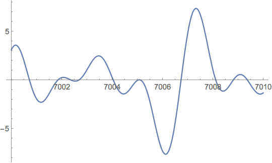
As we know if the maximum of \(Z(t)\) near \(t=7005\) were negative, then RH would be false. This is why Lehmer pointed to this pair of zeros as a quasi-counterexample to RH.

Later other researchers found many other quasi-counterexamples. These are pairs of zeros that are very close to each other in relation to those around them.

This is what carries the information about prime numbers. The zeros of the sine are the points \(\pi n\) with \(n\) integer. They are so ordered that they carry practically no information, we can describe them in one line. But the zeros of \(\zeta(s)\) are the opposite, sometimes close together sometimes far apart and all in no apparent order.

The movement of the zeros

Zeros determine the function \(H _t(x)\). Csordas et al. proved that $$H_t(x)=H_t(0)\prod_{j=1}^\infty \Bigl(1-\frac{x^2}{x_j(t)^2}\Bigr).$$ The differential equation of the zeros informally indicates that the zeros \(x_n(t)\) repel each other. If in some region the zeros are more concentrated they will tend to move towards less dense areas as \(t\) grows. Moving towards an equilibrium position which is represented by an arithmetic progression.

In fact \(e^{a^2 t}\sin(ax)\) has zeros \(\pi n/a\) in arithmetic progression and verifies the retrograde heat equation.

In their paper Csordas, Smith and Varga study the situation of Lehmer’s quasi-counterexamples and find that if two zeros of a function \(H_t(x)\) are very close in relation to the nearby zeros, then they tend to move further apart as \(t\) increases. That is, when \(t\) increases the zeros tend to be placed in arithmetic progression.

(We should say that this is only a local matter in the sense that the zeros of \(H_t(x)\) for a fixed \(t\) tend to be more and more densely placed as \(x\) grows).

The paper by Csordas et al. contains a precise definition of Lehmer Pair. The pair of real consecutive zeros \(x_k(0)<x_{k+1}(0)\) of the function \(H_0(x)\) is said to be a Lehmer pair if the difference \(\Delta_k=x_{k+1}(0)-x_k(0)\) satisfies the inequality\(\Delta_k^2\cdot g_k(0)<4/5\) where $$g_k(0)=\sum_{j\ne k, k+1}\Bigl(\frac{1}{(x_k(0)-x_j(0))^2}+\frac{1}{(x_{k+1}(0)-x_j(0))^2}
\Bigr).$$

The point of the definition is that if we have a Lehmer pair we can give a lower bound of the Bruijn-Newman constant \(\lambda_k\le \Lambda\), being \(\lambda_k\) a known function of \(\Delta_k\) and \(g_k(0)\).

By using the previous data, given by Andrew Odlyzko, Csordas et al. find a Lehmer pair \((x_{1115578}, x_{1115579})\) showing that  \(\Lambda\ge-4.379\cdot 10^{-6}\). This bound improved on previous ones and has been exceeded several times. The latest bound, obtained in 2011 by the same method and using a better Lehmer pair, is \(\Lambda\ge-1.15\cdot 10^{-11}\).

From the evolution of the zeros we should say that the most extreme case, when \(H_t(x)\) has a real double zero, it follows that \(\Lambda\ge t\). We also see that if \(H_0(x)\) had, as the numerical data seem to suggest, infinite Lehmer pairs with \(g_k(0)\ge 0\), it would follow that \(\Lambda\ge0\). That explains Newman’s sentence. If \(\Lambda\ge0\) means that \(H_0(x)\) would have all zeros real, but just barely.

Hugh Montgomery and the correlation of pairs of zeros

In order to understand the work of Rodgers and Tao we must go back in time to describe Montgomery’s surprising results on the distribution of zeros of zeta.

In number theory, expressions that equate a sum in primes with a sum in zeta zeros are called explicit formulas. To study the correlations between the zeta zeros Hugh Montgomery (1972) starts from one of these explicit formulas $$\sum_{p^k\le x}\frac{\log p}{p^s}=-\frac{\zeta'(s)}{\zeta(s)}+\frac{x^{1-s}}{1-s}-\sum_\rho\frac{x^{\rho-s}}{\rho-s}+\sum_{n=1}^\infty \frac{x^{-2n-s}}{2n+s}.$$ Montgomery assumes the Riemannian hypothesis and considers for each large \(T>0\) the set of the ordinates of the zeros \(0<\gamma_n\le T\), taking \(0<\gamma_1<\gamma_2<\cdots\). As \(T\) increases these zeros become increasingly dense, so he normalises them by taking the proportional numbers \(x_n=\frac{\gamma_n\log T}{2\pi}\). The new numbers \(x_n\) are distributed like the \(\gamma_n\) but their mean distance is \(1\). And now study the correlations, that is, the distribution of the \(x_n-x_m\) differences with \(n>m\). The number of these zeros up to the height \(T\) are of the order of \(\frac{T}{2\pi}\log T\). What Montgomery proves is that $$\lim_{T\to\infty}\frac{\text{cardinal}\{(n,m)\colon \alpha<x_n-x_m<\beta\}}{\frac{T}{2\pi}\log T}=
\int_\alpha^\beta\Bigl[1-\Bigl(\frac{\sin \pi u}{\pi u}\Bigr)^2\Bigr]\,du$$

We see that the differences of the zeros are not uniformly distributed but that there are more or less probable differences.

The story has been told many times how the physicist F. Dyson explained to Montgomery that this was the correlation of the eigenvalues of a Gaussian random unitary matrix. This connected with Hilbert-Pólya’s suggestion that the ordinates \(\gamma_n\) of the zeta zeros should be the eigenvalues of a unitary matrix and that this would be the way to a proof of RH. This led to the GUE conjecture (Gaussian Unitary Ensemble) about the distribution of zeta zeros and has since moved research on zeros.

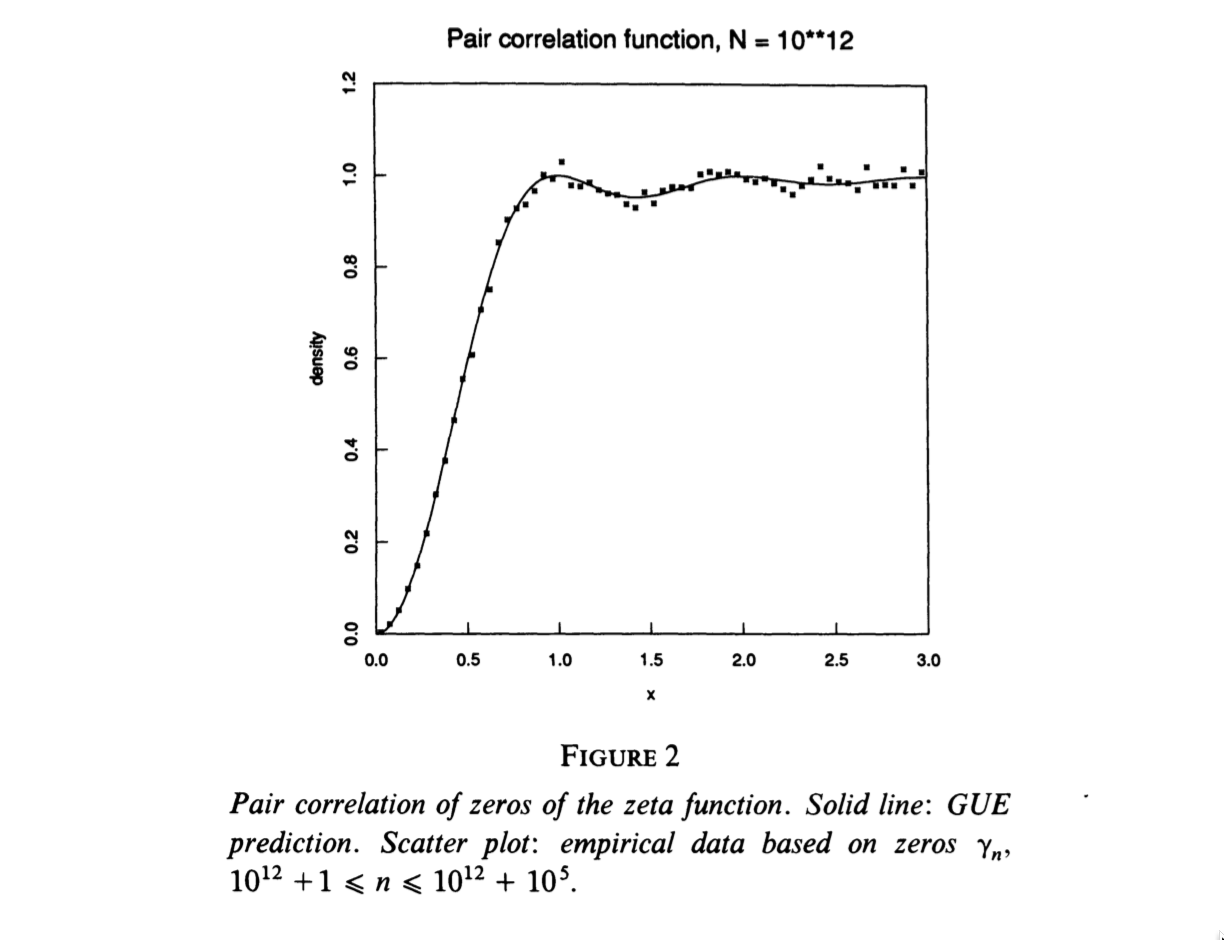
The GUE conjecture is not proven today, but Montgomery’s less ambitious results are proven if we admit RH. There are some spectacular graphs obtained by Odlyzko on this distribution.

Rodgers and Tao’s paper

Rodgers and Tao prove (without admitting any additional hypotheses) Newman’s \(\Lambda\ge0\) conjecture. The proof is by reductio ad absurdum. Suppose \(\Lambda<0\), then by Newman’s result \(H_0(x)\) will have all its zeros real. Therefore RH would be valid. And we can admit it in the whole reasoning by reductio ad absurdum.

Since \(\Lambda<0\) the equation of motion of the \(x_n(t)\) has a time interval in which to act from \(t=\Lambda\) to the value \(t=0\). It is therefore reasonable to think that its zeros will be relatively close to the equilibrium position. But this contradicts Montgomery’s results.

 

Of course, the above assertions have to be made quantitative. Not easy, Rodgers and Tao’s paper is 44 pages long.

They first refine the analysis of Csordas et al. and come up with an upper bound on the space between consecutive zeros.

$$\log\frac{1}{|x_{n+1}(t)-x_n(t)|}\ll (\log n)^2\log\log n,\qquad n\ge n_0, \quad \Lambda/2\le t\le 0.$$
This almost allows them to define the Hamiltonian of the system $${\mathcal H}(t)=\sum_{n\ne m}\log\frac{1}{|x_{m}(t)-x_n(t)|}.$$ The reasoning is complicated. In the end they come to prove that
$$x_{n+1}(0)-x_n(0)=\frac{4\pi+o_{T\to\infty}(1)}{\log T}$$ for a fraction \(1-o(1)\) of \(n\in [T\log T, 2T\log T]\). Since these \(x_j(0)\) are proportional to the ordinates of the zeros of \(\zeta(s)\), this implies that the gaps between the zeros of the zeta function are rarely much larger than their mean value. While the opposite is claimed by Montgomery in [2]. The full proof of Montgomery’s claim can be found in the work of Conrey et al. [4]. They prove that for any \(\lambda>0.77\) there exists a constant \(c(\lambda)>0\) such that at least a proportion \(c(\lambda)\) of \(n\le T\log T\) satisfy $$x_{n+1}(0)-x_n(0)\le \lambda\frac{4\pi}{\log T}.$$ The contradiction proves that \(\Lambda\ge0\).

 Polymath 15

The above results at first glance suggest that the proof of RH is now further away than ever. If RH is true, the slightest perturbation of the \(H_0(t)\) function will cause complex zeros to appear. Possibly there is either some double zero or an infinity of increasingly extreme Lehmer pairs.

This irregularity of zeros has always been the main difficulty in proving RH. There seems to be no asymptotic approximation to \(\Xi(t)\) or \(Z(t)\) that implies that the zeros are real, or even that most of the zeros are real. Current methods fail to prove even that 50% of the zeros of \(\zeta(s)\) are on the critical line.

However, Tao does not seem to have dropped the ball. On 24 January Tao proposed a new Polymath project.

Polymath 15 project: Upper bounding the de Bruijn-Newman constant

At this stage it is known that \(0\le \Lambda<1/2\). de Bruijn proved that \(\Lambda\le 1/2\) and H. Ki et al. proved that in fact \(\Lambda<1/2\). Tao proposes to improve the upper bound of \(\Lambda\).

Tao states that he does not expect to prove the Riemann hypothesis in this way, but advancing our knowledge of \(H_t(z)\) functions and improving the upper bound of \(\Lambda\) do seem realistic goals.

I do think it could be an interesting path. Any function \(H_t(x)\) with \(t>0\) is essentially simpler than \(H_0(x)\). It would suffice to prove that they all have real zeros to get RH proved. It may be that every \(H_t(x)\), with \(t>0\), is essentially simpler than all RH. And there have never been such good mathematicians behind it.

About Polymath

The Polymath Project is a collaboration between mathematicians to solve important and difficult problems through cooperation on the web. The project began in January 2009 when Tim Gowers invited his readers on his blog to upload partial ideas and progress towards the solution of a particular problem he proposed. The success of the project meant that new projects continued to be added. Tao’s current project is number 15. Information about them can be found on the wiki: wiki for polymath projects.

 

Learn more

Terence Tao’s blog explaining his result.

A post on “La ciencia de la mula Francis” blog.

Wikipedia entry on the de Bruijn-Newman constant.

Information on the retrograde heat equation.

The paper of B. Rodgers and Terence Tao

Finally the works cited above:

[1] de Bruijn, N. G.  The roots of trigonometric integrals.  Duke Math. J. 17, (1950). 197-226.

[2] Montgomery, H. L. The pair correlation of zeros of the zeta function. Analytic number theory (Proc. Sympos. Pure Math., Vol. XXIV, St. Louis Univ., St. Louis, Mo., 1972), pp. 181–193. Amer. Math. Soc., Providence, R.I., 1973.

[3] Newman, C. M. Fourier transforms with only real zeros. Proc. Amer. Math. Soc. 61 (1976), no. 2, 245-251 (1977).

[4] Conrey, J. B.; Ghosh, A.; Goldston, D.; Gonek, S. M.; Heath-Brown, D. R., On the distribution of gaps between zeros of the zeta-function. Quart. J. Math. Oxford Ser. (2) 36 (1985), no. 141, 43-51.

[5] Odlyzko, A. M. On the distribution of spacings between zeros of the zeta function. Math. Comp. 48 (1987), no. 177, 273-308.

[6] Csordas, G.; Smith, W.; Varga, R. S., Lehmer pairs of zeros, the de Bruijn-Newman constant \(\Lambda\), and the Riemann hypothesis.  Constr. Approx. 10 (1994), no. 1, 107–129.

[7] H. Ki;  Y. O. Kim;  J. Lee, On the de Bruijn-Newman constant, Advances in Mathematics, 22 (2009), 281–306.

[8] Rodgers, B.; Tao, T., The de Bruijn-Newman constant is non-negative, arXiv 1801.05914, January 2018.