
We have already discussed in these pages that Mathematics is the language of the Universe as well as the essential role it plays in the scientific method. In this entry we are going to look at this last part in a more detailed way. To do so, we will discuss what a physical theory is and we will look at a couple of representative examples. First of all, we have to say that Physics is the Science that studies Nature and that it is based on measurements and experimental observations of the reality that surrounds us, that is, on quantifying or describing the different natural phenomena by means of quantitative expressions or numbers and, from them, proposing theories that explain them.
The measurable or observable properties considered in physics are called physical magnitudes: for example, length, speed, energy, etc. The object or set of objects to be studied is called a physical system: e.g. a material particle, an atom, a car, etc. When we know the measurements of a system that determine it biunivocally, we say that the system is in a given state.
Thus, the objectives of any physical theory are, in general, the following:
1. To describe the state of the physical system, i.e. to give a quantitative (mathematical) representation of the state that uniquely defines it.
2. To know the dynamics of the system, i.e. given an initial state at time \(t_0\) to know its temporal evolution for \(t>t_0\).
3. To predict the results of the measurements of the physical quantities of the system.
From a formal point of view a physical theory is in general constituted by:
1. Formalism: A set of symbols and rules of deduction from which propositions and statements can be deduced. In general, all theories begin by establishing a certain number of axioms commonly known as postulates.
2. Dynamic law: A certain relation (or relations) between some of the main objects of the formalism that allow predicting future events.
Up to this point, the astute reader will discover that there is hardly any difference between a mathematical theory and a physics theory. The main difference lies in the following:
3. Physical interpretation: A set of rules that allow experimental values to be assigned to some of the symbols of the formalism.
This is what some of us call “the method of reductio ad absurdum of Nature” or “putting one’s feet on the ground”. It is this third point that makes the scientific method work, since it is thanks to it that we will know whether or not a theory will be able to explain the phenomena that we are trying to understand and describe using the techniques described in points 1 and 2. A mathematical theory has a life of its own, it is governed by its own laws, often aesthetic, but not a physical theory, which has to pass through the filter of its usefulness when describing natural phenomena.
As an illustrative example we will choose the Newtonian mechanics of a material particle moving in one dimension. Let us imagine that we have a particle of mass \(m\) moving in a single direction under the action of a certain force \(F\) (if you like, you can think of a steel marble rolling along a rail on the ground) as shown in the figure below:

The state of our particle will be determined by its position and velocity. The different quantities that we can measure at each instant of time are, among others, the position of the ball \(x(t)\) at each instant of time \(t\), its velocity \(v(t)\), the acceleration \(a(t)\), the kinetic energy \(T=\frac12 m v^2(t)\), etc. Before continuing, it is worthwhile to digress briefly to explain what some of the above-mentioned quantities are.
According to the Merriam-Webster Dictionary velocity is the rate of change of position along a straight line with respect to time. Likewise, acceleration is a magnitude that expresses the rate of change of velocity with respect to time. If we want to express this variation in mathematical terms, we need one of the most important concepts in mathematics: the concept of the derivative of a function. To define the derivative we can again turn to the Merriam-Webster, which says that the derivative is the limit of the ratio of the change in a function to the corresponding change in its independent variable as the latter change approaches zero. So, if \(x(t)\) represents the distance travelled by our particle, we will have that the velocity is
\(v(t)=\displaystyle\lim_{\Delta t\to0}\frac{x(t+\Delta t)-x(t)}{\Delta t}\)
and acceleration would be the derivative of velocity, i.e. the second derivative of position. The concept of the derivative has a long and interesting history since it was introduced into mathematics independently by Newton and Leibniz in the 17th century when they both developed what we know today as the Differential and Integral Calculus, but this is another story.
Let us now continue with our example. The second thing we must have in our physical theory is a dynamic law, which in this case is none other than Newton’s 2nd Law. This law states that \(F=m\cdot a\) where \(a\) is the acceleration of the particle, that is, the acceleration of a particle is proportional to the applied force and inversely proportional to the mass of the particle. If we denote by \(x(t)\) the position of our particle then Newton’s second law takes the form \(F(t)=m \ddot{x}(t)\) which is a differential equation (since its unknown is not an algebraic quantity but a function, in this case the displacement of our particle). Here we have used Newton’s notation for derivatives: \(v(t)=\dot{x}(t)\), \(a(t)=\dot{v}(t)=\ddot{x}(t)\) , which is the usual one in many Physics texts, but not in Mathematics texts where Leibniz’s notation is more usual. To solve the differential equation obtained (which is often complicated and is not the aim of this entry) we must know the values of \(x(t)\) and its derivative \(\dot{x}(t)=v(t)\) at a certain instant of time \(t_0\), that is, the so-called initial conditions of the problem (in our example, the initial position and velocity of our particle) which we denote by \(x_0=x(t_0)\) and \(v_0=v(t_0)=v(t_0)\), respectively.
Let us now look at two very simple particular cases. The first is when the force is a constant force. Then our differential equation becomes \(\ddot{x}(t)=F/m=a\). Using the rules of Calculus (which we are not going to explain here) it follows that\(v(t)=\dot{x}(t)=v(t_0)+a t\) and \(x(t)= x(t_0)+v(t_0)t+a t^2/2\). That is to say, if a constant force acts on the body, the space it travels depends quadratically on time. From the above formula it follows, in particular, that if \(F=0\), then \(a=0\), and therefore \(v(t)=v(t_0)\), that is, the body moves with constant velocity, as Galileo established years before (and which is, in turn, the first of Newton’s three Laws of Mechanics).
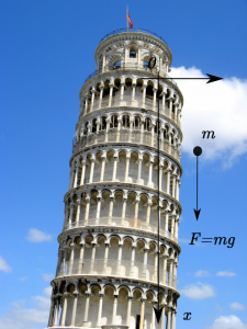
Let us now examine the problem of a body falling from a certain height. Suppose, for example, that we drop our steel ball from the tower of Pisa (as the legend says Galileo did in his day). Since the force acting on the ball is the force of gravity which is equal to \(F=m\cdot g\), where \(m\) is the mass and \(g\) is a constant, usually called the acceleration of gravity, then, using again Newton’s second law we obtain that \(a=g\).
Assuming that we drop our ball from rest, that is \(v_0=0\), we deduce that the distance \(x(t)\) that the ball travels is written by the formula \(x(t)=g\cdot t^2/2\), that is, the distance travelled is proportional to the square of the time elapsed. This relation was precisely the Law that Galileo described in his work Discourse and Mathematical Demonstrations on two new sciences, specifically in Theorem II, Proposition II of the chapter On naturally accelerated motion Galileo proves that “If a mobile falls, starting from rest, with a uniformly accelerated motion, the spaces travelled by it in any time whatsoever are between them as the square of the proportion between the times, or what is the same, as the squares of the times”.
The second example we are going to consider is that of the physical system known as the harmonic oscillator. An example of this type of system is that composed of a particle of mass \(m\) (our steel marble for example) held to the wall by a spring. A simplified diagram of a harmonic oscillator is shown in the figure below:
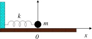
If we stretch the spring, it applies to the ball a force proportional (and in the opposite direction) to the elongation (or deformation) of the spring. Let us assume that the point marked \(0\) in the diagram represents the equilibrium position (i.e. when the spring is neither stretched nor compressed), and let us denote by \(x(t)\) the elongation of the spring. Then, on the ball always acts a force proportional to the elongation whose expression is \(F=- k \cdot x(t)\) being \(k\) a certain constant known as the elastic constant of the spring (the minus sign is due to the fact that the force always opposes the movement of the sample ball as the reader can verify if he tries to stretch or compress a spring). Therefore, the equation of motion is, according to Newton’s second law, \(m \ddot{x}(t) = – k \cdot x(t)\), or equivalently, \(\ddot{x}(t) + \omega^2 \cdot x(t)=0\), where \(\omega^2=k/m\). The general solution of this equation is a sinusoidal function of the form \(x(t)=A’sin(\omega t+delta)\). This function represents the oscillations of the particle around the equilibrium position \(0\), where \(A\) is the amplitude and \(\omega\) is the frequency of the oscillation. In the following figure we see a graphical representation of this function which shows, in addition to the period of the oscillation \(T=2\pi/\omega\), the amplitude of the oscillation itself:

In the following animation we show a representation of what happens to our steel ball. For simplicity we have chosen the case when we lengthen the spring to a distance \(A\) from the equilibrium point and then release it so that its initial velocity is zero.
As we can see, the ball oscillates between the values \(x_{min}=-A\) and \(x_{max}=A\), points where the ball stops and changes the direction of its motion. At these two points the elongation \(x(t)\) is the largest possible (in absolute value) and equal to \(A\) while its velocity is zero. On the contrary at the equilibrium position \(x(t)=0\) the ball has the highest possible velocity (in absolute value) equal to \(\omega A\).
For the case of the harmonic oscillator we will calculate the total energy of the particle. For this we will use the formula
\(E=\frac{m\cdot v(t)^2}2+\frac{k\cdot x(t)^2}2.\)
If we substitute in this expression the solution we found before we obtain for the total energy of our oscillator the following value: \(E=\frac{ k A^2}2\). Note that this value does not depend on time so we are in the presence of a system where energy is conserved.
Although very simple, these examples show very well how a physical theory is constructed. We should mention that an important feature of the harmonic oscillator that follows from the above formulae is that its energy, which we have already seen is conserved over time, is a function that varies continuously with the amplitude of the oscillation (the latter only depends on the initial values of the \(x(t)\) and \(v(t)\)). This is a property of almost all known macroscopic systems. It came as a surprise when it was discovered that in many microscopic systems (such as atoms and molecules, for example) the energy ceased to be continuous and became a jump function. But this is the story of quantum mechanics, which we will discuss another time.
So we see that mathematics plays an essential role in the construction of any physical theory, indeed it is an essential part of it, for without mathematics there is no physical theory as such. But their relationship is much deeper. A very good description of this is given by the great Soviet mathematician Vladimir I. Arnold. Arnold who in his magnificent essay On Teaching of Mathematics wrote “In the middle of the twentieth century it was attempted to divide physics and mathematics. The consequences turned out to be catastrophic. Whole generations of mathematicians grew up without knowing half of their science and, of course, in total ignorance of any other sciences. […] mathematics that is cut off from physics is fit neither for teaching nor for application in any other science”
Leave a Reply