
In several previous posts we have commented that Mathematics is the language of nature (see here) and we have also seen that it plays a fundamental role in the scientific method (see here). That there is a close relationship between mathematics and the world around us, that apparent mystery of which Einstein and Wigner spoke, is also discussed in this other post. This relationship between mathematics and the world around us is also described in a masterly way by the brilliant mathematician John Von Neumann (1903-1957) in his article The Mathematician, published in 1947, in which he states:
I think that it is a relatively good approximation to truth – which is much too complicated to allow anything but approximations – that mathematical ideas originate in empirics, although the genealogy is sometimes long and obscure. But, once they are so conceived, the subject begins to live a peculiar life of its own and is better compared to a creative one, governed by almost entirely aesthetical motivations, than to anything else and, in particular, to an empirical science.
In this entry we want to show one of the most representative examples of what Von Neumann says, specifically we will show how a mathematical theory born from Physics can take on a life of its own and give rise to mathematical studies that are not only interesting, but that have changed Mathematics itself. Our example is related to the so-called trigonometric series, usually called Fourier series.
A trigonometric series is an infinite series of the type
\(\displaystyle S=\displaystyle\frac{a_0}2+\sum_{n=1}^\infty a_n \cos (n x)+b_n \sin (n x),\)
where \(a_n\) and \(b_n\) are certain numerical sequences given beforehand. For example
\(\displaystyle\sin(x)+\frac{\sin 3x}{3}+ \frac{\sin 5x}{5}+ \frac{\sin 7x}{7}+\cdots\)
Historically, trigonometric series such as the one above appeared in the 18th century when trying to solve certain physical problems related to the vibrations of a string. This video shows these vibrations very well.
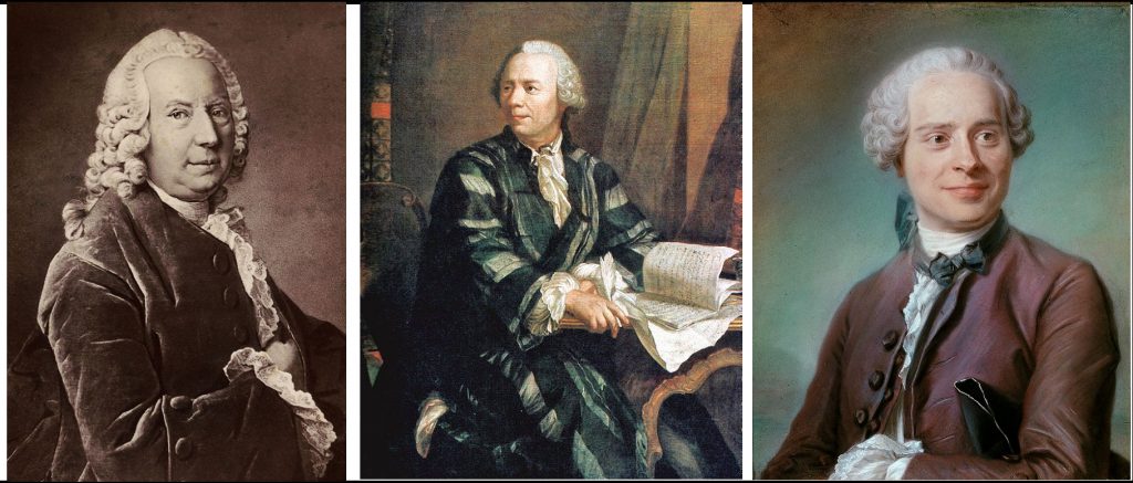
This problem was first treated in some detail by Jean Bernoulli (in 1727), and later by his son Daniel Bernoulli (in 1733). It was also considered by Leonhard Euler (in 1736), although it was not until Jean d’Alembert’s work of 1746 (published in 1749) that a significant advance was made.
d’Alembert, from Newton’s equations of mechanics, derived what we know today as the wave equation
\(\displaystyle\frac{\partial^2 y(x,t)}{\partial t^2}=v^2 \frac{\partial^2 y(x,t)}{\partial x^2},\)
is some constant (the propagation velocity of the wave). Also d’Alembert found that the solution of the wave equation could be written in the form \(y(x,y)=\phi(x+vt)+\psi(x-vt)\), where \(\phi\) and \(\psi\) are arbitrary functions provided they have partial derivatives of order two. In particular he proved that if the string is fixed at its ends and has length \(l\) and at the initial instant has the form defined by a certain function \(f(x)\) then the most general solution had the form
\(y(x,t)=\frac12 \phi(x+vt)-\frac12 \phi(vt-x),\)
where \(\phi\) is a twice differentiable function (i.e. it has two derivatives), periodic with period \(2l\) and uneven, and it must be such that at \([0,l]\) $ \(\phi(x)=f(x)\). Both d’Alembert himself and Euler (who published an article on the subject in 1948 shortly after reading d’Alembert’s work) arrived at the above expression, the latter being the definitive solution of the problem of the vibrating string.
Some controversy arose over this last statement, since Daniel Bernoulli in an article of 1753 (published in 1755) defended by means of physical arguments that the general solution was not the formula of d’Alembert and Euler but the infinite series
\(\displaystyle y(x,t)=\sum_{m=1}^\infty c_m \sin\frac{m\pi x}{l} \sin\frac{m\pi at}{l}.\)
Note that from the above formula it follows, in particular, that if \(t=0\), then
\(\displaystyle y(x,0)=f(x)=\sum_{n=1}^\infty c_n \sin\frac{n\pi x}{l}\),
that is, the function \(f(x)\) (which a priori is arbitrary), must be able to be represented, at least in the interval \([0,l]\), as a trigonometric series. This property is not at all trivial to prove and the search for the answer generated a huge number of interesting mathematical problems and theories, some of which we will mention shortly.
Returning to Bernoulli’s work, he argued that since he had infinite coefficients \(c_n\) in his formula, this would allow him to represent any function without any problem, although he had no method to do so (in the case of an infinite sum). Today it is obvious that this is not true in general, since the infinite number of coefficients Bernoulli had at his disposal is not comparable with the number of points where the function is defined: one is numerable or countable (the number of coefficients \(c_n\)) while the other, the number of points of \(f\) in the interval \([0,l]\) is not, but for that we would have to wait for Cantor and his studies on set theory and transfinite numbers, a theory which was motivated precisely by the problem of the uniqueness of the representation of a function by a Fourier series (of which the Bernoulli series is a particular case).
Before continuing it is worth noting that if we have a development like the one above we can, formally, multiply both members of the equation by \(\sin\frac{k\pi x}{l}\), and integrate from \(0\) to \(l\). If we use that
\(\displaystyle \int_0^l \sin\frac{k\pi x}{l} \sin\frac{m\pi x}{l}dx=0, \mbox{ if } m\neq k,\, m=0\, k=0,\)
and equal $latex\frac{l}2$, if \(m=k\), we obtain the following value for the coefficients \(c_n\)
\(\displaystyle c_n=\frac{2}l \int_{0}^l f(s) \sin\frac{n \pi s}{l} ds.\)
This fact was (essentially) realised by Euler in 1777, although the result was published after his death in 1793.
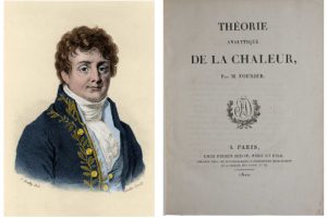
The next relevant step in this history is due to Joseph Fourier. Fourier was interested in one of the most interesting problems of the early 19th century: the transmission of heat through a body. Although Fourier’s first paper was presented in 1807, it was not until 1822 that his seminal work was published, which has undoubtedly been one of the most influential mathematical treatises in history: Théorie analytique de la chaleur (Analytical theory of heat).
Based on physical principles, Fourier derived what is today another of the fundamental equations of physics-mathematics: the heat equation. If we restrict ourselves to a single dimension, the equation describing the propagation of heat through a homogeneous bar of length \(l\) has the form
\(\displaystyle \frac{\partial u(x,t)}{\partial t}=a^2 \frac{\partial^2 u(x,t)}{\partial x^2},\)
where \(u(x,t)\) is the temperature of the bar at the point \(x\) and at time \(t\). To the previous equation we will have to add an initial condition (temperature distribution) \(u(x,0)=f(x)\) and two boundary conditions \(u(0,t)=g_1(t)\) and \(u(l,t)=g_2(t)\), which for simplicity we will take equal to zero.
To solve the heat equation Fourier used the method of separation of variables introduced by d’Alembert in his study of the wave equation. The idea is to suppose that the solution admits a representation in the form of separate variables \(u(x,t)=X(x)T(t),\qquad X(x)\not\equiv0,\quad T(t)\not\equiv0.\)
Substituting the above into the original equation and after some not complicated calculations Fourier deduced that the general solution of the heat equation was given by the series
\(\displaystyle u(x,t)=\sum_{n=1}^\infty b_n e^{-\frac{a^2\pi^2n^2 t}{l^2}} \sin \frac{n\pi x}l, \)
with \(b_n\) certain numbers to be determined.
Note that if \(t=0\) then, the initial condition gives us the formula
\(\displaystyle f(x)=\sum_{n=1}^\infty b_ n \sin \frac{n\pi x}l,\)
which is the development in sines of a function.
That is to say, once again we come back to the problem of the development of a function in trigonometric series that we have already discussed above. Here, however, Fourier uses an inventive method to find the form of the coefficients which leads him to the expression
\(\displaystyle b_n=\frac{2}l \int_{0}^l f(s) \sin\frac{n \pi s}{l} ds\).
Although the way in which Fourier derived the above integral representation for the \(b_n\) coefficients left much to be desired from the point of view of rigour, Fourier, unlike his predecessors, realised its importance (and generality). For example, Fourier argued that it was enough for the curve \(f(x)\sin \frac{n\pi x}l\) to have area, which made sense to him for a large number of functions that did not even have to be continuous, and might not even have an analytic representation (i.e. a single formula). From this Fourier concluded that any function in \([0,l]\) admitted a representation in series of sines. But he went further, for on the basis of several concrete examples he claimed that the representation was always valid in \([0,l]\) no matter what happened outside that interval. He further claimed that two functions could perfectly well be identical in a given interval, and different outside it. This fact was of vital importance because many mathematicians of the time did not consider this possibility feasible.
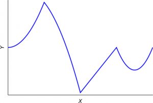
In support of these mathematicians, we should mention that in Fourier’s time the concept of a function was not yet clear. In fact, there were different ways of understanding what a function was, the most widespread being the notion that a function was expressed by a single formula. Euler was one of the first to defend that a function could be described by several formulae, which is what today we call a piecewise defined function, like the one in the following figure:
Fourier’s work was essential in clarifying the concept of function. It was unthinkable before Fourier’s work that a function could be like the one we know today as the Dirichlet function, which took values equal to 1 at all the rational points on the real line and 0 at the irrational points and which, apart from not being continuous at any point, was impossible to represent graphically.
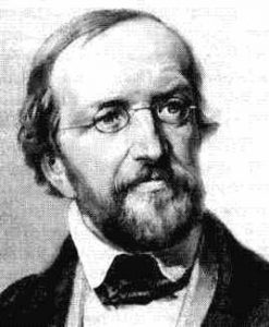
In fact Peter Gustav Lejeune Dirichlet is credited for the modern definition of function:
A function is a rule such that every \(x\) value of a (numerical) set is matched (no matter how) by the value \(y\), in which case \(y\) is said to be a function of \(x\) and is written as \(y(x)\).
But let us move back to Fourier’s work. After considering the developments of functions in sines, Fourier analyses developments in cosines and then studies the representation of a function in the interval \([-l,l]\). After analysing various examples, he deduces that any function can be represented in \([-l,l]\) by the series
\(\displaystyle f(x)=\frac{a_0}{2}+\sum_{n=1}^\infty a_n \cos\frac{n\pi x}{l}+b_n \sin\frac{n\pi x}{l},\)
where
\(\displaystyle a_n= \frac1{l} \int_{-l}^l f(x) \cos {\frac{n\pi x}{l}} dx,\quad b_n= \frac1{l} \int_{-l}^l f(x)\sin{\frac{n\pi x}{l}} dx, \quad n=0,1,2,3,\dots\,.\)
The above development is precisely what we know today as the Fourier series, which represents functions in the interval \([-l,l]\) and their periodic extensions outside this interval.
Note that for the above expressions to make sense, the integrals that define the coefficients \(a_n\) and \(b_n\) must be well defined. In fact, in order to answer the question of which functions admit a Fourier series, a rigorous theory of integration had to be developed, first by Bernhard Riemann and then by Henri Lebesgue’s theory of integration.
If we now assume that given a function \(f\), its Fourier series exists, then the question naturally arises whether the Fourier series really represents the initial \(f\) function. Before answering that question, it is useful to show some simple examples:
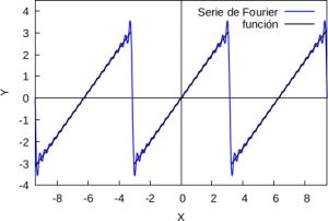
Example 1: Let \(f(x)=x\) be the function \(f(x)=x\) defined on \((-\pi,\pi]\) and let us extend it periodically to the whole real axis. The Fourier development of it is:
\(\displaystyle S_f(x)=2\sum_{k=0}^\infty \frac{(-1)^{k+1}\sin kx}{k}.\)
In the figure below we can see a representation of the first 10 summands of the same. Note that \(f\) is discontinuous at the points \((2k+1)\pi\), \(k=0,\pm1,\pm2,\ldots\) while the partial sums of \(S_f\) are continuous and furthermore \(S_f((2k+1)\pi))=0\).
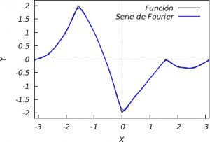
Example 2: Let us now show an example of a function as proposed by Euler. Let \(g\) be defined on \((-\pi,\pi]\) by
\(\displaystyle g(x)=\left\{\begin{array}{ll}\mbox{si}\; x\in[-\pi,\pi/2), \quad & f(x)={{8\,\left(x+ \pi\right)^2}\over{\pi^2}}, \\[3mm] \mbox{si}\; x\in[-\pi/2,0),\quad & f(x)={{5}\over{2}}-\frac12{\left({{4x+3 \pi}\over{\pi}}\right)^2}, \\[3mm] \mbox{si}\; x\in[0,-\pi/2),\quad & f(x)={{4\,\left(x+\pi\right)}\over{\pi}}-6, \\[3mm] \mbox{si}\; x\in[\pi/2,\pi),\quad & f(x)= \frac13{\left( {{4 x-3\pi}\over{\pi}}\right)^2}-\frac13. \\ \end{array} \right. \)
and extend it periodically to the whole real axis. After laborious calculations we can obtain the first 10 terms of the series shown in the figure below:
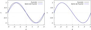
Example 3: Finally let us consider the function \(h(x)=x(x^2-\pi^2)\) in \([-\pi,\pi)\) whose Fourier series is
\(\displaystyle S_f(x)=\sum_{k=1}^\infty \frac{(-1)^{k}\sin kx}{k^3}.\)
The graph shows that even with a single summand the approximation is good.
From the above examples it follows that if the function is good enough the convergence of the series seems to improve significantly so the question arises whether there is any relation between the smoothness of \(f\) and the convergence of its corresponding Fourier series.
One of the first rigorous results on this problem is due to Dirichlet who proved that: If a function \(f(x)\) is a periodic function of period \(2l\), piecewise continuous and bounded, which in one period has a finite number of local maxima and minima and a finite number of discontinuities, then the Fourier series converges to \(f(x)\) at every point where \(f\) is continuous and to the value \(\displaystyle\frac{f(x+)+f(x-)}2 \) at the points of discontinuity where \(f(x+)\) and \(f(x-)\) are the limits on the right and on the left, respectively, that is, the limits when \(h>0\) such that \(\displaystyle f(x+)=\lim_{h\to0} f(x+h)\) and \(\displaystyle f(x-)=\lim_{h\to0} f(x-h)\),thus inaugurating the search for sufficient conditions that would ensure the convergence of the Fourier series.
Let us return to the question of what conditions \(f\) must satisfy in order to have a Fourier series. Dirichlet himself realised that not for any function the series could be defined. In fact he used the function that bears his name and that we mentioned before to conclude that not for any function the integrals are going to be defined. One might think that it would be enough if \(f\) were integrable (the integral of the absolute value of \(f\) existed) according to Lebesgue’s definition. The answer was not long in coming. On the one hand Andrey Kolmogorov proved in 1926 that there were integrable functions whose Fourier series diverged at all points and on the other Jean-Pierre Kahane and Yitzhak Katznelson in 1966 proved that there were continuous functions whose Fourier series diverged in a sufficiently small set (called the set of null measure). The most general answer known today is due to the Swedish mathematician Lennart Carleson who proved in 1966 that if a function is square integrable (i.e. if \(|f(x)|^2\) is integrable), then its Fourier series can be defined and it converges to the function at almost every point in the interval except perhaps one of null measure. This was generalised by Richard Hunt in 1968 to \(L^p\) functions with \(p>1\), i.e., when \(|f(x)|^p\) is integrable. Although with the Carleson-Hunt Theorem the problem of convergence of Fourier series is practically solved, there are still attempts to generalise them to intermediate spaces of functions.
As the reader will have noticed, in order to solve the physical problem of how a string vibrates or how heat is transmitted in a body, it was necessary to develop an immense number of areas of mathematics, which began to… live a peculiar life of their own, governed by almost entirely aesthetic motivations, … as Von Neumann said in his article.
I cannot end this post without writing how Von Neumann concludes the thoughts I transcribed at the beginning of this entry. Von Neumann continued his statement in this way:
As a mathematical discipline travels far from its empirical source, or still more, if it is a second and third generation only indirectly inspired by ideas coming from “reality” it is beset with very grave dangers. It becomes more and more purely aestheticizing, more and more purely l’art pour l’art. This need not be bad, if the field is surrounded by correlated subjects, which still have closer empirical connections, or if the discipline is under the influence of men with an exceptionally well-developed taste. But there is a grave danger that the subject will develop along the line of least resistance, […] In other words, at a great distance from its empirical source, or after much “abstract” inbreeding, a mathematical subject is in danger of degeneration.
And what is the solution proposed by good old Johnny?
Whenever this point is reached, it seems to me that the only remedy is the rejuvenating return to the source, the re-injection of more or less directly empirical ideas.
It is easy to deduce from von Neumann’s words that this apparent dependence of mathematics on reality, which frightens so many mathematicians, is not at all degrading for Mathematics, nor should it be hidden, but rather the opposite: it should be enhanced.
Recommended readings:
F. Javier Duoandikoetxea Zuazo, 200 años de convergencia de las series de Fourier. Gaceta de la Real Sociedad Matematica Española, Vol. 10, No. 3 (2007), pp. 651-677.
Edward B. Van Vleck, The Influence of Fourier’s Series upon the Development of Mathematics. Science, New Series, Vol. 39, No. 995 (Jan. 23, 1914), pp. 113-124
Leave a Reply