
In this post we will continue the story we started in the previous one: the story of a certain dark cloud shadowing the clear skies of Classical Physics. As we narrated there, it all started with the problem of how hot bodies absorbed and emitted heat. The first plausible theoretical explanation of what the radiation spectrum of a black body looked like (a model developed to solve the problem) was due to the physicist Wilhelm Wien who gave a theoretical explanation in 1896 to the formula found experimentally by Friedrich Paschen that same year. The Paschen-Wein formula is written as follows
$$ u(\omega,T)=\alpha \omega^3 e^{-\beta \omega/T},$$
where \(u(\omega,T)\) is the energy density per unit volume and frequency \(\omega\) emitted by a black body, \(T\) is the temperature and \(\alpha, \beta\) certain constants.
This formula reproduced very well the experimental results for large \(\omega\) frequencies, but failed miserably to explain what happened for small frequencies. In the latter case Lord Rayleigh in 1900 had found that \(u(\omega,T)\) should be proportional to \(\omega^2\) and to \(T\), that is, \(u(\omega,T)= a {\omega^2} T,\) which led to the so-called “ultraviolet catastrophe”, since adding up all the contributions of each of the frequencies meant that the energy density of a black body would be infinite, something that clearly made no sense. As we mentioned in the previous post, Max Planck was the one who finally managed to solve the problem, and he did so by introducing a revolutionary concept: the “quanta” of energy.
Let us try to give an outline of Planck’s reasoning. To get to Wein’s formula, Planck assumed that the black body was made up of “resonators“, which were a kind of electrical oscillators whose oscillation frequencies coincided with the frequencies of electromagnetic radiation (the way in which the oscillator interacted with the radiation was related to the phenomenon of resonance, a phenomenon that had been known for a long time). It should be noted that at the end of the 19th century, the composition of matter as we know it today (atoms consisting of a nucleus with electrons “spinning” around it) had not yet been established, so Planck’s assumption was not entirely unreasonable. The first thing Planck did was to explain how his resonators absorbed and emitted radiation, devoting several papers to the subject between 1895 and 1896. In these papers Planck also had another goal: to define the thermodynamic concept of entropy in mechanics and electromagnetism in a “rational” way. But what is entropy? Before we go any further, let’s try to explain what entropy is.
Entropy is a concept introduced by 19th century physicists in order to write correctly and completely the famous laws of Thermodynamics (specifically the German physicist and mathematician Rudolf Clausius was the one who introduced it in 1850), although it was Ludwig Boltzmann (who we talked about in the previous post) who, when developing statistical mechanics, gave it the mathematical formulation (and the physical interpretation) that we use today and that involves probabilities. And it was precisely this idea that Planck (and others) disliked, because a probabilistic argument implied the non-determinism of physical laws. The concept of entropy is a mathematical concept with many subtleties. One of the usual interpretations is that entropy is a mathematical quantity that measures the degree of disorder (or order if you prefer) of a physical system. This can create some confusion, for example: where is there more order, in a glass of water, or in a glass with a bunch of ice chunks in it (many people answer that the ice chunks in a glass are more disordered than the water left in the glass after the ice chunks melt). To be serious, to answer this question properly, we would first of all have to define somehow what order is in a physical system.
Let us look at a “relatively” simple way of understanding the concept of entropy. For this we will have to resort to what is nowadays known as Boltzmann’s formula. According to this formula the entropy \(S\) of a system of particles is expressed by the formula \(S=k \ln \Omega\), where \(k\) is a positive constant and \(\Omega\) is the number of “microstates” of the system. Let’s make this clear with a simple example. For simplicity let us imagine that we have a system with four particles confined in a box. Let us now imagine that we know that all four particles are to the left of the box (which we will call state A). The only possibility to have such a state (four particles to the left) is represented in the following figure
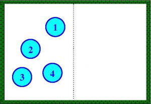
That is, state A can only consist of a single “microstates”. If we now know that the state of our system is that there are three on the left and one on the right (state B), then there are four possible ways (four “microstates”) for this to occur:
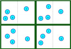
It is natural to think that in our example state A is more ordered than state B. If we use Bolztmann’s formula, then state A has an entropy equal to \(S=k \ln 1 =0\) less than state B which is equal to \(S=k \ln 4\). Let us now impose that for our four-particle system each “microstate” is equally probable, i.e. each microstate occurs with equal probability. So, it is clear that it is four times more likely to find the system in state B than in state A, so if we have four particles in the box it is much more likely that the system is in the higher entropy state (state B) than in the lower entropy state (state A). In fact, the chance of finding our system in a state with two particles on the left and two on the right is 6 times greater than all of them being on the left. If instead of having 4 particles we have 100 then the state when all 100 are on the left has only one possibility, while the state of having 50 and 50 is possible in \(10^{29}\) ways, that is, it is almost certain that our system is in a state closer to the state of 50 and 50 than in the state of 100 on the left (imagine it happens in a room where there are \(10^{27}\) particles). In other words, all systems tend to the state of maximum entropy by pure probability (there are many more states with particles scattered on both sides than with particles concentrated on one side). If we now say that one state is more disordered than another if there are more different ways of obtaining that state from its “microstates”, then it is clear that the state 2 and 2 (or 50 and 50) is more disordered than 4 and 0 (or 100 and 0). Precisely one of the ways of writing the Second Principle of Thermodynamics is to say that every thermodynamic process tends to maximum entropy, or, in other words, that every physical system tends to be as disordered as possible (in the sense of the previous definition).
It was all this probabilistic stuff, plus the fact that he was not clear how to use it in the context of electrodynamics, that Plack did not like about Boltzmann’s theory. And not only Planck. In fact, the rejection of his kinetic theory (which implied the assumption that gases were made up of small particles – atomic theory – in constant motion, something that was not experimentally determined at the end of the 19th century and which we will return to on another occasion) by a large part of the scientific community may have been one of the causes of Bolztmann’s suicide in 1906.
Let us move on. Apart from the probabilistic question above, there was also another tricky issue. For Boltzmann (as for Maxwell, whom we also discussed in the previous post) gases were made up of particles that collided with each other according to the laws of Newton’s classical mechanics. But then a serious problem arose, as pointed out by Planck’s assistant in Berlin, Ernest Zermelo (and yes, he is the same Zermelo of set theory and mathematical logic, to whom we owe the controversial but very useful axiom of choice). The problem was that a few years earlier, in 1890, Henri Poincairé had proved that any mechanical system such as the one Boltzmann proposed (consisting of many particles whose motion obeyed the laws of Newtonian mechanics) would sooner or later (though it might take forever) return to the same state from which it started (or to any of the states it might have been in at some point). In other words, Boltzmann’s statistical mechanics described processes that were irreversible according to thermodynamics (for example, the process of diffusion of a gas in a room is irreversible, since if we initially have all the gas in one corner of a room, it will always be dispersed throughout the room and will never concentrate again in the corner of the room), but the very basis of his theory rested on Newtonian mechanics, which was itself deterministic and therefore could only describe reversible processes, as Poincaré had proved.
But let us return to our story. Planck spent several years studying how the concept of entropy could be used in the context of electromagnetic radiation using his resonators and introducing a concept he called “natural radiation”, and published several papers up to the early 1900s. Among the results he published in 1900 was his contribution to the problem of the emission spectrum of a black body, assuming, as already mentioned, that it was composed of its resonators. In fact, Planck’s proof of the Paschen-Wein formula was quite simple and more elegant than Wein’s own, and as already mentioned, it corresponded very well with the experimental results of the moment. Now, it was well known that the Wein formula worked very well in the high-frequency region of the spectrum, but what about the low-frequency region? In the low-frequency range, there were hardly any experimental results until the first half of the 1900s. The first precise measurements of the energy density for the black body in the low-frequency region were made by two German physicists Heinrich Rubens and Ferdinand Kurlbaum. On 7 October 1900 and before publishing their experiments, Rubens himself discussed with Planck during a visit to his home his experimental results for low frequencies, which, according to his own (Rubens’) words, fitted perfectly with the formula deduced by Lord Rayleigh that same year, i.e. that for high temperatures and long wavelengths (i.e. low frequencies) \(u(\omega,T)= a {\omega^2} T\). Planck immediately set about to modify his proof of Wein’s formula to try to accommodate the new experimental results that Rubens had just told him. That same evening (7 October 1900) Planck sent Rubens his deduction of a new formula for the energy density \(u(\omega,T)\) and Rubens confirmed that the new formula fitted nicely with his experimental results. The formula that Planck derived was as follows
$$ u(\omega,T)=\frac{a \omega^3}{ \exp\left({\frac{ b \omega}{kT}}\right)-1 }$$
which has an extremely interesting property: if \(\omega\) is small then \(u(\omega,T)\sim \omega^2 T\) which agreed with Rayleigh’s formula and if \(\omega\) was very large, Wien’s formula was recovered.
On 9 October 1900 Kurlbaum presented the experimental results at the meeting of the German Physical Society and during the discussion Planck announced that he had found an improvement of Wein’s formula, a formula that agreed very well with experiments over the whole range of wavelengths (or frequencies) of the electromagnetic spectrum. After that session, it seemed that Lord Kelvin’s second little cloud had been eliminated forever from classical physics, for the expression for the energy distribution of blackbody radiation had been found, but…
Yes, dear reader, there is always a “but”. In his reasoning, Planck had made an assumption about the mathematical expression of the black body entropy that was not supported by any physical theory (it is, as we now call it, a phenomenological theory), so he decided to find a rational (i.e. rigorous) justification, from first principles, as laid down in what we call Newton’s Programme. Planck was convinced that all his previous work on resonators could help him to solve this last stumbling block. Although it is difficult to give an idea of Planck’s reasoning without using higher mathematics, let us at least try to give an intuitive idea of his reasoning. Since Planck used certain expressions for entropy, he decided to put aside at least momentarily his dislike for the use of probabilities and delve deeper into Boltzmann’s work.
The first thing Planck did after rereading Boltzmann’s work was to write the entropy formula \(S=k \ln \Omega\) that we saw earlier for a set of elements, where \(\Omega\) is the number of permutations of the different elements that make up the system and that did not change the macroscopic state of the system. In other words, Planck recovered Boltzmann’s probabilistic argumentation. How was Planck able to assume the probabilistic hypothesis that he had so strongly rejected a short time before? He himself explained it 30 years later in a letter to the physicist Robert Williams Wood written on 7 October 1931:
Briefly, what I did can be described simply as an act of desperation. By nature I am peaceful and opposed to uncertain adventures. However, I had already struggled unsuccessfully for six years with the problem of the equilibrium between radiation and matter without reaching any successful result. I was aware that the problem was of fundamental importance in physics and I knew the formula describing the energy distribution in the normal spectrum [of a black body]. Therefore, a theoretical interpretation had to be found at any cost, no matter how high it might be.
Indeed, the formula to which Planck refers here was the one he had found after Rubens’ visit to his house. Using the experimental data, this formula could be written as
$$ u(\omega,T)=\frac{8\pi h \omega^3}{c^3}\frac{1}{ \exp\left({\frac{ h\omega}{kT}}\right)-1 },$$
where \(h=6.55 \cdot 10^{-27} (erg\cdot seg)\), \(c\) is the speed of light and \(k\) is Boltzmann constant.
Armed with Boltzmann’s expression for entropy, Planck applied it to black body radiation. He assumed that the black body consisted of \(N\) resonators with \(\omega\) frequency. So, in Planck’s words
If E is considered to be an infinitely divisible quantity, then the distribution of E over the N resonators can be done in infinitely many ways. However we will consider E to be composed of a finite number of equal parts and use for this purpose the natural constant \(h=6.55 \cdot 10^{-27} (erg\cdot sec)\). This constant multiplied by the \(\omega\) value of the frequency of the resonators, gives us the number of \(\epsilon\) energy elements to distribute over the N resonators.
The rest is much more technical, but everything was already said: the energy E could not be divided infinitely, it had to be absorbed and radiated in finite portions determined by the frequency \(\omega\) of the radiation (which corresponded to the frequency of the corresponding resonator). This was the price that had to be paid for not collapsing the rest of the laws of thermodynamics (according to Planck it was either that or give up the inalienable laws of thermodynamics).
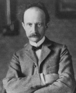
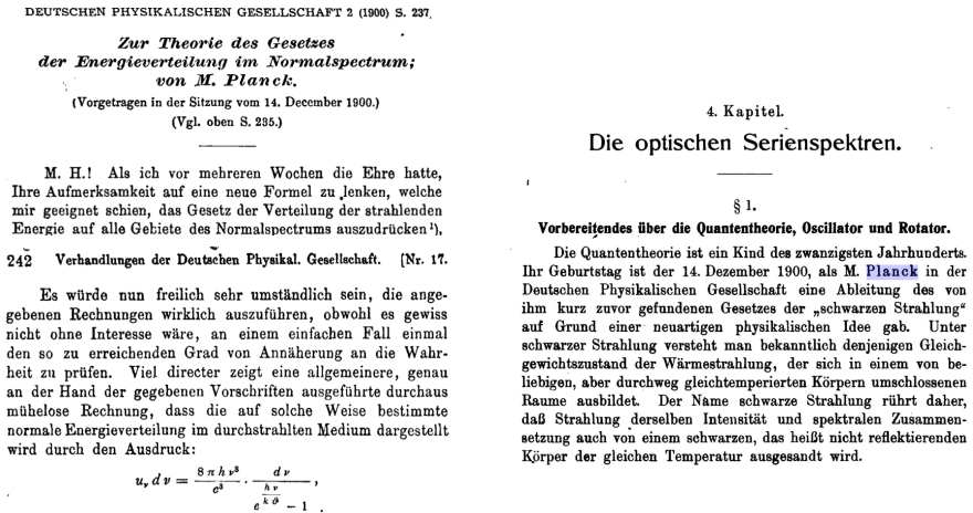
Planck presented his results on 14 December 1900 at the meeting of the German Physical Society in a paper entitled “Zur Theorie des Gesetzes der Energieverteilung im Normalspektrum” (On the theory of the law of energy distribution in the normal spectrum), which was later published in Verh. d. Deutsch. Phys. Ges. (2) 2, 237-245. On that day, as the great German theoretical physicist Arnold Sommerfeld wrote years later in his 1919 book Atombau und Spektrallinien (Atomic Structure and Spectral Lines), quantum theory was born and with it a new physics that would change the world. Planck’s quantum theory was not to everyone’s liking, but in the years that followed, Planck himself and other physicists proposed simpler ways of deriving the formula, and a large number of experiments were carried out that confirmed the veracity of Planck’s formula. The “Planck action quantum” (as it was later christened) had arrived in physics, and it was here to stay. What seemed like a mathematical artifice became one of the most disturbing ideas of the early 20th century, as the protagonist of our next story, Albert Einstein, later revealed.
Learn more:
Chapter 1 of J. Mehra y H. Rechenberg, The Historical Development of Quantum Theory, Vol 1. The Quantum Theory of Planck, Einstein, Bohr and Sommerfeld: Its Foundation and the Rise of Its Difficulties 1900-1925, 1982 Springer-Verlag New York Inc.
A 5-minute introduction to thermodynamics can be found in this video and to entropy in this one.
Leave a Reply