
In mathematics, modelling is an attempt to extract the significantly important aspects of a real situation and translate them into mathematical expressions and equations. Except in very simple processes, what is obtained will never be accurate, because the model cannot necessarily capture the whole reality or all the variables involved, nor incorporate all the initial data from which it starts. But it can be used to study the process and to foresee, in some way, how the introduction of specific measures may cause its future evolution to vary.
In particular, this is what happens with the development of epidemics, and this is what we are going to try to do here using the SEIR epidemiological model, well adapted to the COVID-19 coronavirus epidemic. For this modelling, we will incorporate variations in order to take into account the control measures being adopted. We will not try to make an actual prediction with specific numbers (in particular, this would require more medical and political data than we have at our reach), but to show the influence of the measures on the development of the epidemic. We only want to show qualitative trends – with a more or less technical explanation of the mathematical tools used in the calculations and the uncertainties inherent in the process, which all epidemiologists encounter – , not to give quantitative forecasts of what the future of the epidemic will look like. (This post is an excerpt from a longer article that can be found in full here).
SEIR epidemiological model
For our modelling we will use the SEIR model (an adaptation of the SIR model, proposed by W. O. Kermack and A. G. McKendrick in 1927). In a population of fixed size \(N\) in which an epidemic has broken out and spread by contagion, at time \(t\) individuals can be in four different states:
Susceptible: \(S(t)\),
Exposed: \(E(t)\),
Infected: \(I(t)\),
Recovered: \(R(t)\).
The SEIR model is well adapted to the behaviour of the coronavirus epidemic because, for this disease, in addition to those susceptible to infection, those already infected and those who have recovered, we must also take into account those who are exposed, i.e. individuals who carry the disease but who, being in their incubation period, do not show symptoms and cannot yet infect others (we must be precise with what we are denoted: if an individual does not show symptoms but can infect others we count them in \(I(t)\), not in \(E(t)\)).
In the SEIR model we have three parameters: \(\beta\), called transmission rate, so that \(1/\beta\) measures the probability of a susceptible becoming infected when it comes into contact with an infected person; \(\gamma\), called recovery rate, so that the average recovery period is \(1/\gamma\); and \(\sigma\), so that \(1/\sigma\) is the average incubation time. The first two parameters define the parameter \(R_0=\beta/\gamma\) which is called the basic reproduction rate and represents the number of new infections produced by an infected person if the entire population is susceptible.
The differential equations of the basic SEIR model are
$$\begin{cases} S'(t) = -\beta S(t)I(t)/N, \\E'(t) = \beta S(t)I(t)/N – \sigma E(t), \\I'(t) = \sigma E(t) – \gamma I(t), \\R'(t) = \gamma I(t).\end{cases}.$$
Epidemiological model for COVID-19 with containment measures
Using the SEIR method, and following what has been published in [1], to model the evolution of the COVID-19 coronavirus we will take the following values for the parameters: \(\gamma= 1/5\), \(\sigma= 1/7\). It is more complicated to estimate \(\beta\); in particular, because it is not known how many asymptomatic infected people there are who may be infecting others.
Several studies of disease behaviour in China before drastic population isolation measures were adopted (such as the one cited above [1]) suggest that the value of \(\beta\) could be between 0.59 and 1.68 (in units of days\({}^{-1}\)), which would give a \(R_0\) between 2.95 and 8.4, in both cases quite high (a recent paper in the Lancet [3] takes \(R_0=2.68\)).
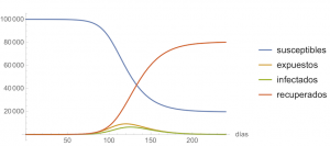
Taking then \(\beta=1\) and assuming we have a population of \(100\,000\) people, in which there is one infected at the beginning, the evolution of the epidemic modelled with the differential equations of the SEIR model for 120 days would be as shown in the figure below.

With not very different parameters the specific values of the functions \(S(t), E(t), I(t)\) and \(R(t)\) would vary, but the appearance of the graphs would be similar.
So far we have considered that the infection rate \(\beta\) is constant. But this parameter can be artificially adjusted if containment measures (protection and isolation) are taken, and if the population accepts and complies with them. Thus, several studies have been carried out with time-varying \(\beta\). For example (see [2]), with a decreasing function over time in the form
$$\beta(t) = \beta_0 \Big((c_0-c_b)e^{-r_1t} + c_b\Big)$$
donde \(\beta_0\) sería la tasa de infección sin medidas de contención y las constantes \(c_0\) y \(c_b\) aluden a las tasas de contacto (fruto de los aislamientos de la población); o, también (véase [1]),
$$ \beta(t) = \beta_0 (1-\alpha(t)) \left(1 – \frac{D(t)}{N}\right)^{\kappa},$$
where \(\beta_0\) is the infection rate without measures, \(\alpha(t)\) (with values in the interval [0, 1]) is the result of government actions, \(D(t)\) is the public sense of risk as a consequence of critical cases and known deaths, and \(\kappa\) measures the intensity of individuals’ reaction.
Typically, \(\alpha(t)\) is a constant function in pieces (measurements are taken at specific times), and some estimates (cited in [1]) suggest that one can take \(\kappa=1117.3\) (although it seems somewhat ridiculous to take a value with five digits of precision, that is the value obtained in previous studies for other situations and, in the absence of other information, that is what they use).
The idea of the \((1-D(t)/N)^\kappa\) factor with a high \(\kappa\) is that, when concern is high, the factor is very close to 0, people isolate themselves even voluntarily and \(\beta(t)\) is very small; conversely, the factor is close to 1 and has little influence if social concern is low. As the Chinese and Western socio-political realities are not the same, one can hardly think that we can use their same parameters, but we can use their same modelling ideas. As an estimate for \(D(t)\) we can think of 5% of cases as serious and thus (without over-complicating the equations) take \(D(t) = 0.05I(t)\) and a high but more moderate \(\kappa\), say, \(\kappa=100\).
If containment measures had been taken from the beginning, the evolution of the epidemic would have been very different. For example, if, in the equation for \(\beta(t)\) above, \(\beta_0=1\), and \(\alpha(t)\) had had the constant value 0.5, the evolution of the epidemic would have been as shown in the figure below.
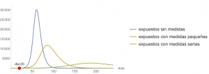
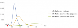
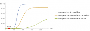
Once again, these are estimates, it is impossible to know the future, but it is possible to analyse how the measures affect the evolution of the epidemic; in particular, the changes in the value of \(\alpha\). We will show how the epidemic would evolve in three different scenarios. Specifically, the figure below compares how the evolution of \(S(t)\), \(E(t)\), \(I(t)\) and \(R(t)\) would change if no containment measures were applied (i.e. as in the first figure) or if these measures were started on day 20, that is with
$$\beta(t) = \begin{cases} \beta_0, & \text{ if $t < 20$},\\ \beta_0 (1-\alpha) \left(1 – {0.05I(t)}/{N}\right)^{\kappa}, & \text{ if $t \ge 20$},\end{cases} $$
with \(\beta_0 = 1.0\) and \(\kappa=100\). In turn, we analyze two different values of \(\alpha\): \(\alpha=0.4\) (minor measures) and \(\alpha=0.7\) (severe measures). It is clear that the containment measures are indeed effective, that they allow the “peak” to be smoothed out, and that they move it away in time. It is also clear that the effect of the measures is not immediate, but takes days to become apparent. What \(\alpha\) will be obtained with specific measures taken by a government is impossible to know beforehand, it can only be estimated a posteriori in view of what has happened; but, whatever the effect, it will be positive, and, if the daily evaluation of epidemiological data shows that it is not sufficient for what is intended to be achieved, the measures can be tightened.

References
[1] Qianying Lin, Shi Zhao, Daozhou Gao, Yijun Lou, Shu Yang, Salihu S. Musa, Maggie H. Wang, Yongli Cai, Weiming Wang, Lin Yang, Daihai He, A conceptual model for the coronavirus disease 2019 (COVID-19) outbreak in Wuhan, China with individual reaction and governmental action, International Journal of Infectious Diseases 93 (2020), 211–216. Published:
March 04, 2020. https://www.ijidonline.com/article/S1201-9712(20)30117-X/fulltext
[2] Biao Tang, Nicola Luigi Bragazzi, Qian Li, Sanyi Tang, Yanni Xiao, Jianhong Wu, An updated estimation of the risk of transmission of the novel coronavirus (2019-nCov), Infectious Disease Modelling 5 (2020), 248–255. Publicado: February 11, 2020. https://www.sciencedirect.com/science/article/pii/S246804272030004X
[3] Joseph T. Wu, Kathy Leung, Gabriel M. Leung, Nowcasting and forecasting the potential domestic and international spread of the 2019-nCoV outbreak originating in Wuhan, China: a modelling study, Lancet 395 (2020), no. 10225, 689–697. Publicado: Jan 31, 2020. https:
//www.thelancet.com/journals/lancet/article/PIIS0140-6736(20)30260-9/fulltext
Buenas! Será posible acceder a el xls con el que se hicieron estos gráficos? Al menos al modelo elemental, sin incluir medidas gubernamentales, etc. Estoy tratando de utilizar el modelo que aquí se explica. Desde ya, muchas gracias
Las gráficas no están hechas con Excel, sino con Mathematica. En el enlace «aquí» al final del segundo párrafo hay un enlace al trabajo completo, y ahí está el código Mathematica para hacer las gráficas.
Buenas noches. Tengo el archivo excel que contiene todos los calculo por si todavia le interesa. Escribame a mi correo maryelgonz@gmail.com
Hola!! Agradecería por favor pudieran compartir el archivo de Excel.
gamartinezch@yahoo.com
Favor de enviarme el archivo Excel a gcorrea@unamad.edu.pe
Hola de Cali, Colombia. También me podrías compartir el excel. mauricio.ledesma@correounivalle.edu.co
Favor de compartir el archivo. Gracias!!!
serias tan amable de compartir tu archivo excel a miliansf@yahoo.es
gracias de antemano
Favor enviar archivo, lmaumm@gmail.com, Excelente análisis. Saludos
Excelente articulo. Agradecería el archivo en excel.
Carlos Guillermo
cbernate@gmail.com
Por favor, puedes compartir tu archivo excel a milenka.ocampo@gmail.com
Muchas gracias!
Saludos
Hola me podrías compartir el archivo en excel, yisus200162@gmail.com
Enviame tu correo y te envio mi modelo en Excel
Buenas, comentar que las personas en período de incubación también producen contagios, lo cual parece no haberse tenido en cuenta.
Por lo demás magnífico!
Se ha tenido en cuenta hasta cierto punto. Pone esto: “(hay que ser precisos con lo que estamos denotando: si un individuo no presenta síntomas pero sí puede contagiar a otros lo contabilizamos en I(t), no en E(t))”. Se podía haber hecho un poco distinto y haber puesto en las ecuaciones que tanto los I(t) como los E(t) contagian, con distintos parámetros (en algunos estudios que hemos visto posteriormente hacen algo similar y la los que contagian sin presentar síntomas los llaman A(t), asintomáticos). ¿Pero qué tasas de contagio ponerles? Uno puede pensar que los que están incubando tienen pocos virus y son menos contagiosos (desconozco si eso es así), pero también que los E(t), como están malitos, todo el mundo lo ve y tienen menos contactos. ¿De dónde sacar estimaciones para los parámetros? Necesitaríamos estimar cuánto tiempo pasa un enfermo incubando sin contagiar, incubando contagiando sin síntomas, y ya con síntomas, y cuánto de contagioso es en cada caso. No le vimos sentido a introducir más tipos de personas con más parámetros de los que no podíamos dar ningún valor aproximado, solo inventárnoslo.
Cuanto menor es la tasa de contagio (o mayores las medidas gubernamentales que la regulan a lo largo del tiempo) mayor es la duración de la epidemia, por lo que parece inviable aplicar medidas de aislamiento o distanciamiento social desde un principio. Me equivoco? Y si no me equivoco, es posible que por esta razón muchos gobiernos hayan tardado en tomar estas medidas?
Es verdad, cuantas más medidas, más lento todo. Sin medidas de ningún tipo en ningún país, se podía haber acabado todo en un par de meses, con el 90% de la población mundial afectada y varios cientos de millones de muertos, y con todos los hospitales del mundo colapsados sin posibilidad de atender a la mayoría de los enfermos graves que les llegasen (me estoy inventado las cifras, pero los órdenes de magnitud no serían muy distintos). Eso sí, esto hubiera sido menos perjudicial para la economía, según nos ha explicado algún digno representante del partido republicano de EEUU, a quien le deseo que no tenga a su madre entre los infectados. La razón por la que los gobiernos han tardado en tomar medidas no la podemos saber, pero supongo que es porque no se creían que iba a pasar algo así (tampoco la gente, realmente), y daban prioridad a la lucha política sobre lo que algunos les estaban diciendo que iba a ocurrir (no cancelar las manifestaciones del 8 de marzo debería estar penado con homicidio imprudente, lo mismo que con el mitin de Vistalegre); eran incluso incapaces de mirar a Italia, por ejemplo.
Es un modelo interesante que permite analizar la fluctuación de progreso de la epidemia bajo unos parámetros básicos. indican una comprensión hacia las posibilidades comunes de propagación. Ojalá la gente comprenda la necesidad de estos modelos.
gracias por el artículo, se agradece la difusión. una pregunta que me surge: a la hora de estimar gamma, hay que tener en cuenta tanto recuperados como fallecidos, no? es decir, un posible estimador de gamma sería la media de fallecidos y recuperados al día respecto al stock de infectados?
Excelente artículo… muy necesario para la comunidad científica
Es muy buena propuesta, que pasa cuando los casos son muy pocos y su “aricion” o registro tienes periodos muy largos?
Muy agradecido por publicar el estudio, en muy aleccionador
Estimada doctora apreciaria mucho acceder a la base excel de los calculos de modelamiento. Estoy ensayando posibilidades para el contexto mio
un saludo
carlos
Estoy tratando de correr la sintaxis de su trabajo pero me sale este mensaje y no logro obtener la primera gráfica igual a la suya para luego cambiar los parámetros por lo de mi país
ReplaceAll::reps: {sol} is neither a list of replacement rules nor a valid dispatch table, and so cannot be used for replacing.
Plot::nonopt: Options expected (instead of PlotLegends\[RightArrow]{susceptibles,expuestos,infectados,recuperados}) beyond position 2 in Plot[{sS[t],eE[t],iI[t],rR[t]}/. sol,{t,0,120},PlotRange\[RightArrow]All,AxesOrigin\[RightArrow]{0,0},AxesLabel\[RightArrow]{días,Null},PlotLegends\[RightArrow]{susceptibles,expuestos,infectados,recuperados}]. An option must be a rule or a list of rules.
Juan Carlos, casi seguro que serán cosas del copiar y pegar desde el pdf. Escríbeme un email a jvarona@unirioja.es y te mando el notebook de Mathematica.
Gracias por compartir el trabajo.Es excelente material.
Muchas gracias por este articulo, los muertos no figuran en esta modelizacion?
Me uno a los agradecimientos por este trabajo.
Tengo una duda, en relación con la definicion del parametro beta. El articulo dice: » beta llamado tasa de transmisión, de manera que 1/beta mide la probabilidad de que un susceptible se infecte cuando entra en contacto con un infectado». En otro momento se le llama con el nombre, ligeramente distinto, de «tasa de infección». Y en otra parte del articulo se dice que «1/beta es el tiempo típico entre contactos»
Mis preguntas son: (1) ¿cómo puede beta tomar valores menores que 1 si su inverso mide una probabilidad? (ref. página 4 del articulo) (2) ¿es o no beta el inverso de una magnitud temporal (como parece el caso en los otros 3 parámetros del modelo SEIR, cuyos inversos se miden en días)?
Un gran trabajo. Gracias por compartir su codigo, he tatado de replicar la primera grafica sin lograrlo, al correr el script, me arroja el siguiente error:
Syntax::bktmop: Expression “NDSolve[{sS'[t]==-beta0*sS[t]*iI[t]/nN,eE'[t]==beta0*sS[t]*iI[t]/nN-sigma*eE[t],iI'[t]==sigma*eE[t]-gamma*iI[t],rR'[t]==gamma*iI[t],sS[0]==nN-iI0,eE[0]==I0,iI[0]==0,rR[0]==0},{sS,eE,iI,rR},{t,0,240}];
<>]” has no opening “[“.Plot::nonopt: Options expected (instead of PlotLegends\[RightArrow]{susceptibles,expuestos,infectados,recuperados}) beyond position 2 in Plot[{sS[t],eE[t],iI[t],rR[t]}/. sol,{t,0,120},PlotRange\[RightArrow]All,AxesOrigin\[RightArrow]{0,0},AxesLabel\[RightArrow]{días,Null},PlotLegends\[RightArrow]{susceptibles,expuestos,infectados,recuperados}]. An option must be a rule or a list of rules. Debe ser error de sintaxis.Por favor me podria ayudar, toda vez que necesito hacer este analisis con los datos de mi pais. De antemano muchas gracias
¡Muy motivador! Agradesco su tiempo y la forma tan didáctica de exponernos el Modelo SEIR.
Estimada Dra. Les felicito por la excelente presentación, muy clara y didactica le agradeceria me hiciera llegar el archivo excel para poder aplicarlo a la realidad de mi región. Desde ya se agradece, cordiales saludos
Buenas
Podrían por favor compartirme el Excel, agradecido por los aportes.
Excelente explicación del modelo, favor le solicito me pueda compartir el excel del modelo.
ME PUEDEN ENVIAR EL EXCEL
Muy buena explicación.
Por favor podría compartir su archivo excel al correo: lualvega@hotmail.com
Por favor compartir el archivo excel a oscarmartinezmichel@gmail.com