How long can the coronavirus last outside our body?

In order to understand the stability of the SARS-CoV-2 coronavirus, both in droplets in suspension and on different contaminated surfaces, the prestigious New England Journal of Medicine [1] has published the first rigorous study under experimental conditions. Briefly, the results show that airborne and surface contact transmission is plausible, as the virus can remain viable and infectious for at least 3 hours in suspension and up to 3 days on surfaces, although the infective capacity depends on the amount of viral particles present. The half-life detected (based on experiments and subsequent analysis) was 66 minutes for droplets in suspension, about 5.5 hours on stainless steel, almost 7 hours on plastic, 3 hours on cardboard and about 45 minutes on copper.

The stability of the coronavirus in aerosols, and on different surfaces, was obtained by calculating the TCID50, which is the dose of virus capable of infecting 50% of the cultures used; in this case, the experiment was carried out on Vero E6 cells, commonly used in experiments. Obtaining the TCID50 is the most frequently used method of quantification and, although it does not represent a specific number of viral particles, it does show the infectiousness of the virus, which is certainly related to the number of viral particles present. Let’s look at it with data from the article: we start from an inoculum \(10^5\) TCID50/ml, which means that when you add 1 ml of inoculum with a dilution of 1:100 000 to, say, six culture plates, three of them become infected; if, after a given time, the value of the infective dose has changed to, say, \(10^2\) TCID50/ml, it means that for three of the six plates to become infected, the dose has to be a thousand times less diluted (from a 1:100 000 dilution to a 1:100 dilution), so we have a thousand times less virus than at the start.

Another simpler example. Suppose we take a sample from a surface contaminated with a virus. We do not know how many viruses are present in this sample, but if we make different dilutions of the sample, we see that with a 1:10 dilution, half of the cultures are infected. After one hour, we take another sample and obtain that the dilution that infects half of the cultures is 1:5. And another hour later, the dilution that infects half of the cultures is 1:2.5. Even if we do not know the absolute amount of virus present, we see that every hour we have to dilute twice as much as the previous one; in other words, we have half the virus in the sample and we have to dilute half as much to have the same effect.

To make the example even clearer, let’s suppose that in that first sample we took, there were 100 viruses stuck together; if the 1:10 dilution is the one that infects half of the cultures, and we start from 20 cultures, then 10 viruses are needed to infect 10 cultures. One hour later we collect another sample and, to infect all 10 cultures, we see that we need to make a 1:5 dilution, which means that we have obtained 10 viruses, infecting 10 cultures out of 20, from a population of 50 viruses; in other words, one hour later we had half the viruses on the surface. After another hour, we had to make a 1:2.5 dilution to the remaining viruses on the surface (2 hours from the beginning) to infect the 10 cultures of 20, which means that those 10 viruses were in a population of 25; that is, another hour later we have half as many viruses (25) as in the previous hour. And so on until we have less than 10 viruses in the sample and it is no longer a sufficient number to infect half of the cultures. As a result, from different samples taken at different times, and from dilutions capable of infecting 50% of the cultures, we obtain that the half-life of the virus is one hour, because the number of viruses decreases by half every hour. Schematically:

100 viruses in sample → 1:10 dilution; 10 viruses infect 10 of 20 cultures.

One hour later:

50 viruses in sample → 1:5 dilution; 10 viruses infect 10 of 20 cultures.

One hour later:

25 viruses in sample → dilution 1:2.5; 10 viruses infect 10 of 20 cultures.

Although with the TCID50 value we do not know the absolute number of viral particles in the sample, we can see how, over time, this value indicates that the amount of virus is decreasing in the sample, and how more (concentrated) doses are needed to have the same infective capacity.

We will now try to explain how we can interpret the results of this study using a very simple mathematical model: the Malthusian model for population growth. Before we start, it is worth noting that the Malthusian model is the simplest model and works very well when you have a sufficiently large population of individuals. Although this model has several shortcomings, it is quite suitable for describing exponential population growth, and as you will see, it is quite useful in the case at hand (an explanation of how this model works can be found here and here).

The initial assumption of the model is very simple: the growth rate of a population of individuals is proportional to the number of individuals. Thus, if we denote by \(p(t)\) the number of individuals in the population at time t, then the equation that models the dynamics of the population is
$$ p′(t)=a p(t) $$
where a is some constant (known as the population growth rate) that we must derive from the experimental data and \(p′(t)\) is the derivative of \(p(t)\). The solution of the above equation is well known: \(p(t)=p_0 e^{a t}\) with \(p_0\) being the initial value of the population at the initial time instant \(t=0\). It is convenient for numerical computations to write the solution in the form

$$ \log (p(t))=\log (p_0) + a t$$

which is the equation of a straight line with slope \(a\). As explained above, the number of viruses is very difficult to know, so another indicator is often used. Given that what we are interested in is estimating the infective capacity of the virus after it has been dropped on a surface, we are going to use as an indicator the value of the TCID50 explained above, that is, instead of taking \(p(t)\) as the number of viral particles (which we do not know) we will take the value of the TCID50. We will assume that both quantities, TCID50 and the virus population, are proportional, so it is to be expected that the behaviour of TCID50 is also exponential (i.e. it follows the Malthusian or exponential law), which is indeed verified from the analysis of the experimental data obtained in [1] as we will see below.

Since the numerical data used in [1] did not appear explicitly in the article, we have obtained them by digitising the plots in panel A of figure 1 of [1] using the WebPlotDigitizer program freely available by clicking here.

Below we summarise the results of the study for four materials: copper, steel, cardboard and plastic.

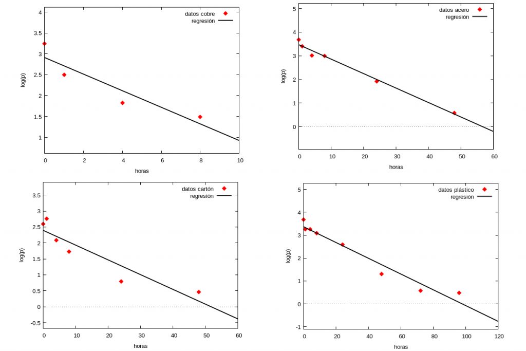
The diamonds in each graph correspond to the experimental data taken from the figures in [1] and the black line represents in each case the corresponding regression line \(\log (p(t))=a t+b\) obtained by the least squares method. In the following table we show the values of \(a\) for the different materials as well as the correlation coefficient (this coefficient gives an idea of how good the least squares estimation is, being better the closer the value is to \(1\)).

$$\begin{pmatrix} \mbox{Material} & \mbox{Slope} & \mbox{Correlation coefficient}\\
\mbox{copper} & 0.198 & 0.92\\
\mbox{steel} & 0.061 & 0.99\\
\mbox{cardboard} & 0.046 & 0.92\\
\mbox{plastic} & 0.034 & 0.97\end{pmatrix}$$

As can be seen in the table above, the correlation coefficient is quite high, which effectively indicates that the dynamics of TCID50 (and thus of the viral particles) follows the Malthusian law as mentioned above and can therefore be used to describe the durability of the virus on different surfaces.

The population half-life can be defined as the time \(T\) it takes for the population to decrease by half. Since \(p(T)/p(0) =1/2 = e^{a T}\), we have \(T=log(2)/(-a)\). Then, given that we have the slopes \(a\) of the regression lines, we can estimate the half-life of the virus on the different surfaces assuming that, as we have already said, this corresponds to the halving of the TCID50 label. The results are shown in the following table:

$$\begin{pmatrix} \mbox{Material} & \mbox{Slope} & \mbox{Half-life (hours)}\\
\mbox{copper} & 0.198 & 3.48\\
\mbox{steel} & 0.061 & 11.31\\
\mbox{cardboard} & 0.046 & 14.98\\
\mbox{plastic} & 0.034 & 20.12\end{pmatrix}$$

If we draw all four regression lines we have the graph

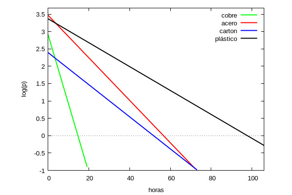
From the above it can be deduced that the virus is capable of remaining infected for longer on plastic than on other surfaces (almost twice as long as on steel or cardboard) and almost 6 times longer than on copper. It should be noted that in [1] the authors estimate the half-life by a different method (using Bayesian inferences) so, although the numerical results do not coincide, they do observe the same general trend: that the virus maintains its infectious capacity for several hours outside the organism and it depends on the material to which it adheres, being on plastic where its half-life is longer. 

In conclusion, the study carried out in [1] (and our own calculations based on the data in [1]) confirm the importance of washing hands thoroughly (soap is enough) when touching plastic, steel and cardboard surfaces, especially if we are not sure that these surfaces are free of contagion. In a future post we will try to explain why soap is good enough and there is no need to worry if you do not have alcohol gel.

Bibliography:

[1] Neeltje van Doremalen, et al. Aerosol and Surface Stability of SARS-CoV-2 as Compared with SARS-CoV-1. The New England Journal of Medicine, March 17, 2020. DOI: 10.1056/NEJMc2004973

This article is co-authored with Prof. Francisco J.Esteban, University of Jaén

If you would like us to send you the maxima programme and the data files you can contact any of the authors: Renato Álvarez-Nodarse (University of Seville) o Francisco J. Esteban (University of Jaén).