Age does matter, but let’s pretend it doesn’t…

We have all been aware these days of the seriousness of the pandemic that has hit us, the dreaded COVID-19. Many aspects of the pandemic have been discussed and analysed in previous posts. In particular, we have seen that the worst forecasts have fallen short. We are already at more than \(18000\) dead in Spain and, unfortunately, we will continue to add more.

In this post we will discuss the importance of age.

Age has a fundamental influence on the number and characteristics of the ailments a person can suffer from. A recent study by the pharmaceutical company Boehringer Ingelheim states that people over the age of \(75\) live with an average of \(3.23\) chronic conditions or diseases, essentially different from those we often see at younger ages. We mainly see bone problems, osteoarthritis and osteoporosis, problems associated with cognitive impairment (Alzheimer’s, Parkinson’s, etc.), benign prostatic hyperplasia, deafness, renal failure, etc.

Our friend and colleague Jacques Simon recently reminded us of a famous quote by General Charles De Gaulle: “Old age is shipwreck”. He was referring to Marshal Pétain and his role as collaborationist head of state from 1940 to 1944. But that statement carries a much more general and deeper message. Sad and painful when we think of our elders, but impossible to escape.

Mathematical models in epidemiology

Mathematical modelling in epidemiology has its main origin in the work of Kermack and McKendrick. They were able to explain and predict how an infectious disease can be transmitted in a population and, from the outset, paid special attention to the role played by age.

Kermack

William O. Kermack (1898-1970) was a Scottish biochemist. At the age of 26, working alone in his laboratory in 1924, he suffered an accident that left him blind for the rest of his life. This did not prevent him from developing a brilliant scientific career. In particular, he was appointed Fellow of the Royal Society of Edinburgh and, some time later, of the Royal Society of London, nominated Doctor Honoris Causa of St Andrews University, and so on. A year after his accident, he married Elizabeth R. Blázquez, daughter of an esparto seller from Águilas (Murcia).

Two more facts:

• Elizabeth had been brought up in England by two aunts of maternal descent. She never learned Spanish. She had 14 siblings whose father and mother, on the other hand, lived all their lives in Spain and never learned English. Thus, to understand each other, the siblings needed a translator.

• Kermack was Professor and then Emeritus at Aberdeen University during the last years of his life. He died suddenly in July 1970, working in his office at Marischal College, Aberdeen University.

McKendrick

Anderson G. McKendrick (1876-1943) was a Scottish military doctor. He began his career as an epidemiologist in India around 1911, “re-discovering” the logistic law. Although his mathematical training was rather elementary, he was gifted with a keen intuition that enabled him to devise different models and to profit from them. Thus, in a 1926 paper, he introduced a partial differential equation, now known as the McKendrick-Von Foerster equation, which models (among other things) the reproductive behaviour of a cell population where age is an important characteristic.

His collaboration with Kermack began in 1927 and generated a general theory for understanding the mechanisms of transmission of infectious diseases.

Go ahead, let’s take age into account

To accurately model the evolution of an epidemic, it is useful to introduce two “times” (two independent variables) into the equations: the usual time variable \(t\), which indicates our living time and an additional variable, denoted \(a\), which we will call the age. This second variable can have two meanings: the “class-age” or time of infection, i.e. the age of the disease, and the “demographic age” or age of the individual.

In the usual models, we look for functions that are interpreted as population densities of susceptible, infected, etc. individuals. Here are some of the simplest ones.

Models based on time of infection

In the original Kermack-McKendrick model, the unknowns are the functions \(S = S(t)\) and \(R = R(t)\), which determine at each given time respectively the total number of individuals susceptible to the disease and the total number of individuals recovered, and the function \(i = i(a,t)\), which gives the infected population density. It is postulated that these functions should verify the equations
$$
\left\{
\begin{array}{l}
S’ = -\lambda(t)\,S, \quad t \in (0,T) \\ i_t + i_a + \gamma(a)\, i = 0, \quad (a,t) \in (0,a_*) \times (0,T)\\ i(0,t) = \lambda(t)\, S(t), \quad t \in (0,T) \\ R’ = \int_0^{a} \gamma(a) i(a,t) \,da, \quad t \in (0,T)
\end{array}
\right.
$$
together with initial conditions \(S(0) = S_0\), \(i(a,0) = i_0(a)\), \(R(0) = R_0\) and the behavioural law $$\lambda(t) = \frac{1}{N}\int_0^{a_*} \beta(a) i(a,t) \,da.$$

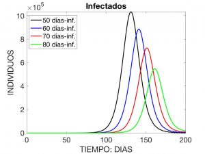
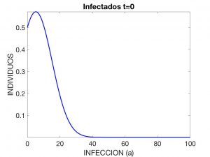
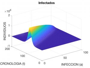
Here, \(\lambda(t)\) is interpreted as the “rate” of infection at time \(t\), \(N\) is the total population, and \(\beta(a)\) and \(\gamma(a)\) are, respectively, the rates of disease transmission and recovery when the age of the disease is \(a\), for example measured in days. It is observed that $$ N \!=\! S(t) \!+\! I(t) \!+\! R(t), \ \hbox{con} \ I(t) \!:=\! \int_0^{a_*} \!i(a,t) \,da $$ and is constant over time (i.e. we accept that no death and no birth occur during the time the disease is active). Figures 3 to 5 visualise the solution to the problem for the following data:
$$
\begin{array}{c}
T = 200, \quad a_* = 100, \quad \beta(a) = 0.05/N, \quad \gamma(a) = 0.7, \\
i_0(a) = 0.57 \times \exp\left(-(a-5.18)^2/200\right), \quad S_0 = N – \int_0^{a_*} i_0(a) \,da, \quad R_0 = 0,
\end{array}
$$
where \(N=4.7 \times 10^7\). These data correspond to the evolution of a contagious disease affecting the Spanish population with an initial distribution of \(10\) infected individuals.

Demographic age

We now assume that the disease has very different effects on individuals depending on their age. Thus, it is convenient to interpret \(a\) as the demographic age, for example measured in years, with \(0 \leq a \leq 100\). Together with \(i = i(a,t)\), we now consider the densities \(s = s(a,t)\) and \(r = r(a,t)\) of susceptible and recovered individuals. It is appropriate to impose the equations $$ \left\{ \begin{array}{l} s_t + s_a + \mu(a)\, s = -\lambda(t)\, s \\ i_t + i_a + (\mu(a) + \gamma(a))\, i = \lambda(t)\, s \\ r_t + r_a + \mu(a)\, r = \gamma(a)\, i \\
i(0,t) = \int_0^{a*} \beta(a) i(a,t) \,da, \ \mbox{ etc.} \end{array} \right. $$
with initial conditions \(s(a,0) = s_0(a)\), \(i(a,0) = i_0(a)\), \(r(a,0) = r_0(a)\). In this system, \(\lambda(t)\), \(\beta(a)\) and \(\gamma(a)\) have the same meaning as in the previous section and \(\mu(a)\) is the mortality rate of the population at age \(a\). We assume that \(\int_0^{100} \mu(a) \,da = +\infty\), i.e. no one survives to ages greater than \(100\) years.

And now we put the newly infected together with the “old-timers” and the young with the old

Let us consider again the initial Kermack-McKendrick model. In the particular case where \(\beta\) and \(\gamma\) are constants, integrating with respect to \(a\) the equations, one easily arrives at the so-called SIR model, an ordinary differential system for \(S\), \(I\) and \(R\): $$ S’ = -\frac{\beta}{N} I \,S, \quad I’ = -\gamma I + \frac{\beta}{N} I \, S, \quad R’ = \gamma I. $$

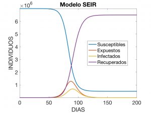
It is common to consider a generalised model, where we add an additional variable \(E = E(t)\) that determines the number of exposed individuals, i.e. incubating carriers of the disease who do not show symptoms and cannot yet infect others. We thus find the SEIR model: $$ \left\{ \begin{array}{l} S’ = -\frac{\beta}{N} I\,S \\ E’ = \frac{\beta}{N} I\,S – \sigma E \\ I’ = -\gamma I + \sigma E \\ R’ = \gamma I \end{array} \right. $$ where (again) \(\beta\) y \(\gamma\) are the transmission and recovery rates and \(\sigma\) is interpreted as the incubation rate of the disease. It is common practice to introduce the notation
$$
\hbox{T}_{\mbox{inf}} := \frac{1}{\gamma}, \quad \hbox{T}_{\mbox{inc}} := \frac{1}{\sigma}, \quad \hbox{R}_0 := \frac{\beta}{\gamma}
$$
and call these three quantities the infection time, the incubation time and the contagion factor. To understand what the solutions look like, we have visualised in Figure 6 the one corresponding to the data
$$
\begin{array}{c}
T = 240, \quad \beta = 0.98, \quad \gamma = 0.34, \quad \sigma = 0.19,\\
E_0 = 1, \quad I_0 = 1, \quad R_0 = 1, \quad S_0 = N – (E_0+I_0+R_0).
\end{array}
$$

with \(N=7 \times 10^6\).

The parameter identification problem

When it comes to solving the preceding systems, we find a greater difficulty: it is not easy to determine the coefficients \(\beta\), \(\gamma\), etc. (be they constants or not) by direct methods, not even in an approximate way.

In practice, we are therefore faced with inverse problems where part of the data are unknown and, in exchange, we have information about what has been happening over a period of time. In theory, this information should allow us to calculate the coefficients and then solve the system and predict the future.

Unfortunately, this process is often fraught with difficulties: on one hand, we have to decide which model best fits the situation; on the other hand, the data are often incomplete and/or affected by significant errors; finally, the mathematical problem behind it may have more than one solution and is generally ill-posed (small perturbations in the information provided often lead to large deviations in the result).

To show that we can do something, we will present below numerical results corresponding to the SEIR model adapted to the evolution of COVID-19 in Spain.

We reason as follows:

• We assume that the values of \(\beta\), \(\gamma\) and \(\sigma\) are piecewise constants: they take an initial value before the confinement date (25 February to 17 March), a second value during the first two weeks of confinement (17 to 29 March) and a third value during the following two weeks (29 March to 10 April), with much more severe measures.

• The known data are $$ T = 160, \quad E_0 = 400, \quad I_0 = 3, \quad R_0 = 0, \quad S_0 = 4.7 \times 10^7 – (E_0+I_0+R_0) $$ and the values \(\tilde{I}_1, \dots, \tilde{I}_m\), \(\tilde{I}_m, \dots, \tilde{I}_n\) y \(\tilde{I}_n, \dots, \tilde{I}_p\), which refer to the three analysed periods.

• With these data we look for constants \(\beta\), \(\gamma\) and \(\sigma\) that minimise the Euclidean distance of the vector \((I(t_1), \dots, I(t_m))\) to \((\tilde{I}_1, \dots, \tilde{I}_m)\); then, the values that minimise the distance from \((I(t_m), \dots, I(t_n))\) to \((\tilde{I}_m, \dots, \tilde{I}_n)\) and finally the values minimising the distance from \((I(t_n), \dots, I(t_p))\) to \((\tilde{I}_n, \dots, \tilde{I}_p)\).

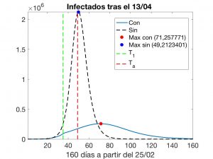
This numerical experiment leads to the results shown in Figures 7 and 8. In the latter, we indicate the instant \(T_1\) at which the second phase of confinement began, the current instant \(T_a\) and also the evolutions that would take place if we accept that the model is adequate. We must not forget that the official data on the number of infected refer to patients detected to date and, for various reasons, have been widely questioned. Thus, we must also “quarantine” (pun intended) the computed solution of the inverse problem.

To learn more

The original papers by Kermack and Mackendrick were republished in the Bulletin of Mathematical Biology:

1. Kermack, W.; McKendrick, A. (1991) “Contributions to the Mathematical Theory of Epidemics, Parts I, II & III”. Bulletin of Mathematical Biology, 53 (1-2): 33-55, 57-87 & 89-118.

For a good understanding of age-structured models, see:

1. Iannelli, M.; Milner, F. (2017) “The Basic Approach to Age-Structured Population Dynamics”. Springer, Dordrecht, The Netherlands.

Other recent works of interest include the following:

1. Li, X.-Z.; Gupur, G.; Zhu, G.-T. (2004) “Analysis of an Age Structured SEIRS Epidemic Model with Varying Total Population Size and Vaccination”. Acta Mathematicae Applicatae Sinica, English Series Vol. 20, No. 1, 25-36.
2. Biswas, B.H.A.; Paiva, L.T.; De Pinho, M.R. (2014) “A SEIR Model for Control of Infectious Diseases with Constraints”. Mathematical Biosciences and Engineering, Vol. 11, No. 4, pp. 761-784.