
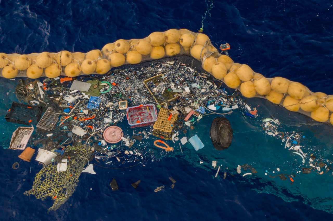
In a previous post (see Plastic waste in the ocean), I referred to a serious environmental problem of our times: the accumulation of plastic debris in the sea in five huge “patches” containing millions of tons of waste. In particular, I wrote about the “Great Pacific Waste Patch” (located between Hawaii and California, with a surface area three times the size of France) and the possible cleaning tool, invented by the young Dutch engineer Boyan Slat (the Ocean Cleanup System 001).
In this post I will discuss the ecological aggravation caused by covid-19, the evolution of the Ocean Cleanup project, and also a relatively simple mathematical formulation of the associated cleanup problem.
The situation is getting worse
The pandemic has worsened the situation in several directions:
-
The use of sanitary equipment has inevitably increased, in particular with regard to single-use plastic. The figures are very alarming and meeting the targets agreed by the European Parliament looks a long way off. Take masks: it is estimated that at least 30-40 tonnes of masks go into the environment every month.
-
In addition, plastic is again being used on a massive scale as an insulating surface, in face shields, in partitions at supermarket checkouts, in disposable products such as gloves and food wrapping, etc. Thus, the environment is seriously endangered. The changes that are taking place in our daily habits do not help either. In particular, we now prefer to use a lot more disposable bags for fear of infection…
-
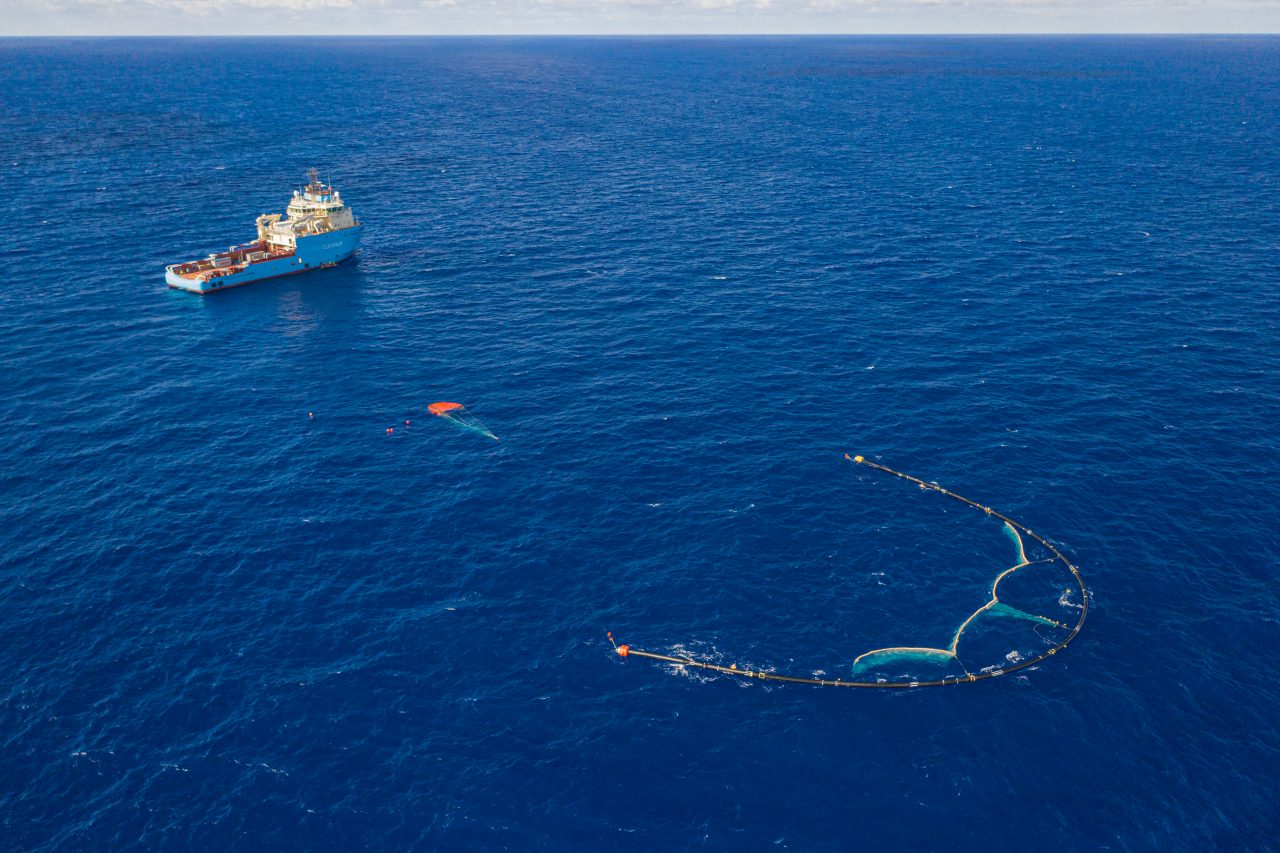
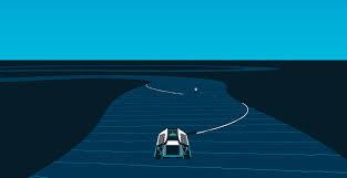
Fig. 2: The OCS 001/B in action Among others, on the beaches of the Soko archipelago (between Hong Kong and Lantau), masks have been seen floating, a clear sign of poor waste management.
- The data also show that many regions on the mainland may also suffer from excessive plastic.
-
To get an idea of how the problem is growing, consider that in 2015, the world generated 380 million tonnes of plastic; by 2050, it is expected to generate more than 1 billion tonnes. If we do nothing, by that date we will curiously have more plastic in the ocean than fish.
Evolution of Ocean Cleanup: Systems 001b and 002, aftertreatment, Interceptors, etc.
The Ocean Cleanup System 001 (OCS 001) consists of a 600 m long flexible structure from which a 3 m high net hangs. It is intended to move the plastic to strategically chosen accumulation points, so that it can be collected at these points and taken to land for further treatment. This tool was tested and put into operation, after 273 scale tests and 6 prototypes, in San Francisco on 8 September 2018. The first campaign lasted until January 2019.
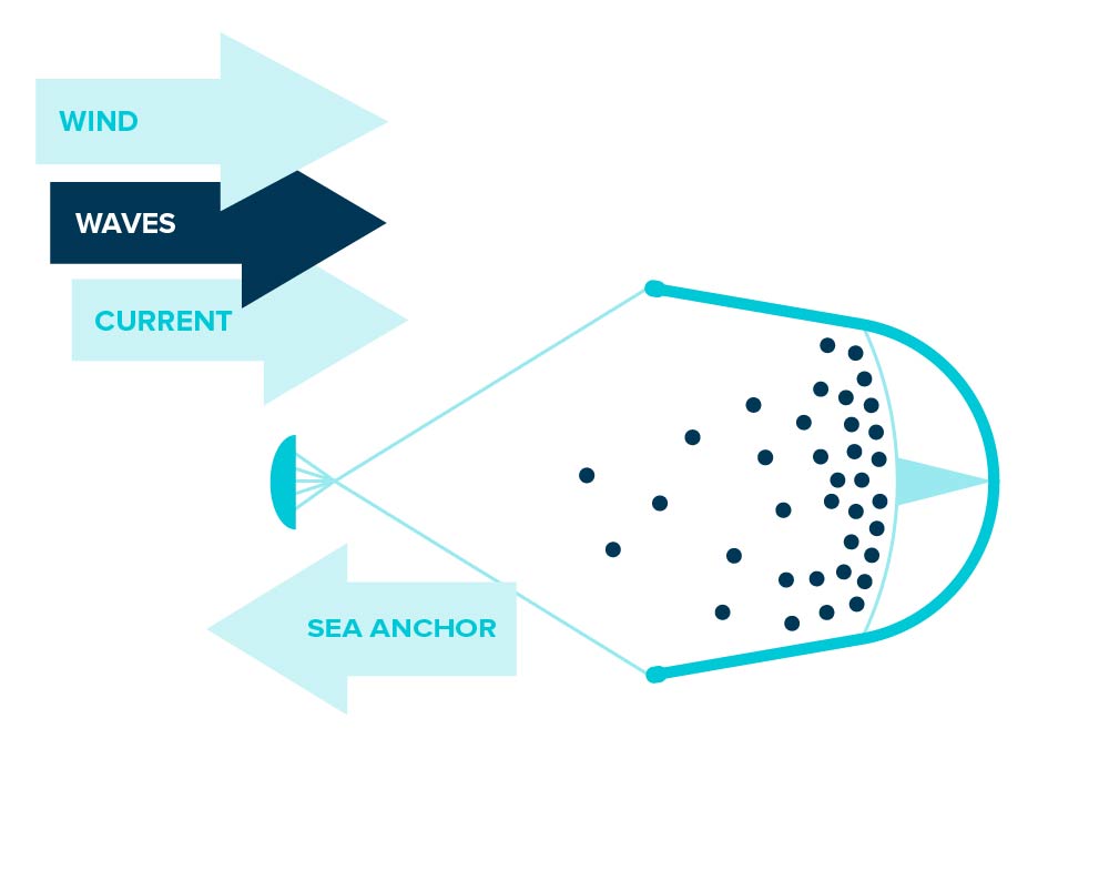
As a result of the tests carried out and in view of the performance, the original system resulted in a modified OCS 001/B system. To improve plastic retention, the speeds at which the structure had to move were adjusted, and to reduce material fatigue effects, the design was slightly modified. The OCS 001/B has been conceived as a modular platform, capable of testing the incorporation of various elements (among others, a parachute to slow down the movement), redefinitions of the dimensions of the structure, etc.
The campaign lasted from June to November 2019, led to significant improvements in performance and resulted in the OCS 002, which is currently being finalised. It is believed that OCS 002 will be key to the large-scale cleaning of the Great Pacific Waste Patch, capable of ensuring efficient collection of plastic waste of all sizes and types.
The Ocean Cleanup project aims to deploy a fleet of approximately 60 such systems over the next 2 years. It is estimated that it would thus be possible to reduce the total amount of ocean plastic by 90 % by 2040.
The plastics trail
Once located, the plastic must follow a process that involves 8 main stages:
-
Capture, secure and seal.
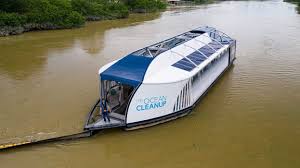
Fig. 4: The interceptor in action -
Transport (at present, no offshore recycling options are available).
-
Pre-sorting. Due to the differences in the various types of plastic, separation is required, essentially of the “fibrous” plastic from the rigid plastic.
-
Recycling, in turn consisting of further sorting and separation, shredding, washing and drying, and extrusion (more precisely, conversion into grains that can then be moulded).
-
Checking (checking for contaminants and reliability).
-
Addition of stabilisers and pigments for the future manufacture of different products.
-
Actual production, based on demand, of new products.
-
Shipment to consumers.
All profits from this process will be reinvested in the clean-up operations of the project.
Interceptors
The Ocean Cleanup project has also resulted in the creation of the Interceptors. These are vessels designed to clean plastic litter from rivers, paying particular attention to those that can lead to significant deposition in seas and oceans (actually, rivers are the main source of plastic pollution, with data showing that 1000 rivers are responsible for about 80% of pollution).
The Interceptors are 100% solar powered and are capable of autonomously extracting plastic and operating in the vast majority of the world’s polluted rivers. They will be the subject of a future entry in this Blog.
A simplified mathematical model for OCS 002
The operation of OCS 002 can be approximately described by a system of partial differential equations (PDEs) of Navier-Stokes type.
We can assume that the system is 2D in space. This means that the equations have to be satisfied in an open set \(Q := \Omega \times (0,T)\), where \(\Omega \subset \mathbf{R}^2\) represents the ocean surface bounded by the structure and \((0,T)\) is the time interval of observation:
$$
\left\{
\begin{array}{l}
\mathbf{v}_t – \nu \Delta\mathbf{v} + (\mathbf{v}\cdot\nabla)\mathbf{v} + {1 \over \rho} \nabla p = \mathbf{h}, \quad \nabla \cdot \mathbf{v} = 0, \quad (\mathbf{x},t) \in Q \\
\psi_t – \kappa \Delta \psi + \mathbf{v} \cdot \nabla \psi = -(f1_\omega) \psi, \quad (\mathbf{x},t) \in Q.
\end{array}
\right.
$$
Here, \(\mathbf{v}\) and \(p\) are, respectively, the velocity field and the hydrostatic pressure of the water, \(\psi\) is interpreted as the pollution density (essentially, the density of plastic in the sea). We will accept that \(\mathbf{h}\) is a given field, linked to environmental conditions (wind, sea currents, additional plastic input, etc.), \(\omega \subset \Omega\) is a small region close to the structure where plastic collection operations take place and \(f\) determines the intensity with which plastic collection takes place. This system must be complemented with boundary and initial conditions for \(\mathbf{v}\) and \(\psi\). Taking a fixed reference frame with respect to OCS 002, among other possibilities is the following:
$$
\left\{\begin{array}{l}\mathbf{v} = 0, \ \ \displaystyle\frac{\partial\psi}{\partial n} = 0, \quad (\mathbf{x},t) \in \Gamma_0 \times (0,T), \\
\mathbf{v} = – \mathbf{a}, \ \ \displaystyle\frac{\partial\psi}{\partial n} = 0, \quad (\mathbf{x},t) \in \Gamma_1 \times (0,T), \\
\bigl.\mathbf{v}\bigr|_{t=0} = \mathbf{v}_0,
\ \ \bigl.\psi\bigr|_{t=0} = \psi_0, \quad \mathbf{x} \in \Omega. \\
\end{array}
\right.
$$
In these equalities, \(\Gamma_0\) and \(\Gamma_1\) represent, respectively, the structure and the open area of the \(\Omega\) domain. The boundary conditions (the first four equalities) indicate that the water sticks to the structure (travelling with velocity \(\mathbf{a}\)) and that it “leaves free” the entrance of debris in the open zone.
In the additional equations and conditions, \(\mathbf{a}\) and \(f\) appear, functions respectively defined on \(\Gamma_0 \times (0,T)\) and \(\omega \times (0,T)\), which play the role of controls: we are free to decide which values they take, which we will logically do by looking for a solution \((\mathbf{v}, p, \psi)\) with a desired behaviour.
In particular, it makes perfect sense to look for \(\mathbf{a}\) and \(f\) such that the associated state \((\mathbf{v}, p, \psi)\) minimises a cost function
$$
J(\mathbf{a}, f) := \frac{a}{2} \int_\Omega |\psi(\mathbf{x},T) – \psi_d(\mathbf{x})|^2 \,d\mathbf{x}
+ \frac{c}{2} \int\!\!\!\!\int_{Q} |f|^2
+ \frac{b}{2} \int\!\!\!\!\int_{\Sigma_1} |\mathbf{a} – \mathbf{a}_d|^2 \,d\Gamma\,dt,
$$
where constants \(a, b, c \geq 0\) and \(a+b+c = 1\) and \(\psi_d\) and \(\mathbf{a}_d\) are (desired) functions previously fixed.
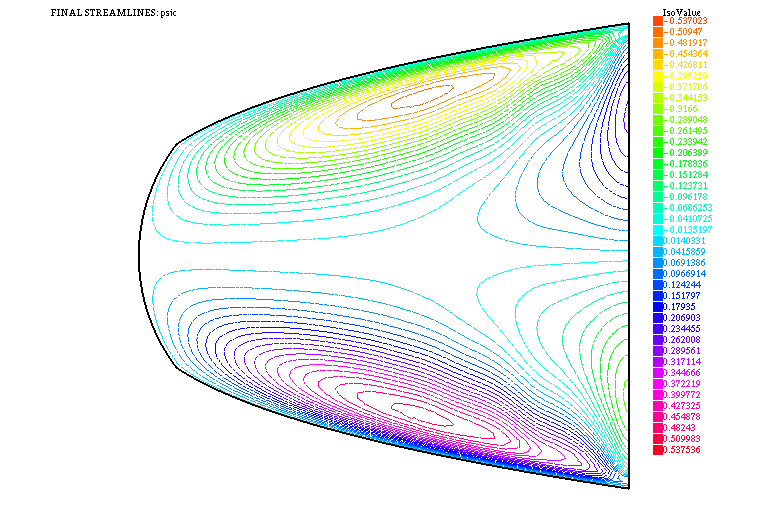
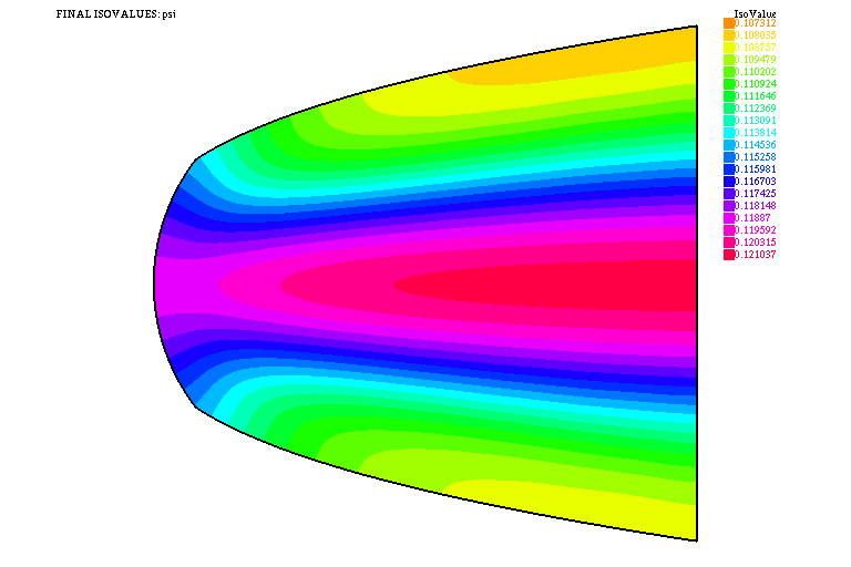
Naturally, for a rigorous analysis of this problem we need to determine the spaces where to choose the control \((\mathbf{a}, f)\), prove that for each admissible pair there exists a unique solution, demonstrate the existence of optimal controls (i.e., admissible pairs that minimise \(J\)), deduce a suitable optimality system, etc. A proper numerical simulation of the above PDE system leads to the results that have been depicted in Figures 6 and 7.
If we go a little further in the analysis of the possible functioning of the system, we can try to make the actions of \(\mathbf{a}\) and \(f\) “independent”, assigning them more than one objective simultaneously. This leads to bi-objective optimal control problems whose solution requires the definition of one or more equilibrium concepts, and also to hierarchical control problems, where one or more objectives are subordinated to others. More details can be found (for example) in the last two references cited below.
Learn more
Details on the Ocean Cleanup project and its evolution:
- B. Slat et al., How the oceans can clean themselves, The Ocean Cleanup, The Netherlands, 2014.
-
https://theoceancleanup.com
On the Interceptor:
-
https://theoceancleanup.com/rivers/
Control problems of Navier-Stokes type systems:
-
R. Glowinski, Finite element methods for incompressible viscous flow, Handbook of numerical analysis, Vol. IX, 3-1176, Handb. Numer. Anal., IX, North-Holland, Amsterdam, 2003.
-
A. Quarteroni, Numerical models for differential problems, Third edition, MS\& A. Modeling, Simulation and Applications, 16. Springer, Cham, 2017.
Hierarchical and multi-objective control problems:
-
F.D. Araruna, E. Fernández-Cara, M.C. Santos, S. Guerrero, New results on the Stackelberg-Nash exact control of linear parabolic equations, Systems & Control Letters, Volume 104, June 2017, Pages 78-85.
-
E. Fernández-Cara, I. Marín-Gayte, Theoretical and numerical results for some bi-objective optimal control problems, Comm. Pure Applied Anal., Volume 19, Number 4, April 2020, pp. 2101-2126.
Site remediation results in a healthier ecosystem which helps the land to experience significant growth. A thriving ecology is necessary if the site is to be restored to its natural beauty.