“Packing” the students in the classroom

At the time of writing this paper we are almost six months into the pandemic (covid-19) and by all indications we will still have some time until Science can find an effective vaccine that will allow us to return to pre-covid life. While we knew little at first about how the disease was transmitted, whether it was just another cold, etc., today, although we are far from being able to say that we understand it fully, we know much more about it (see the July 9 update of the WHO’s scientific summary [1]). For example, one of the facts that has been proven with absolute certainty is that in places with higher concentrations of people (even outdoors) the virus spreads more easily, something, incidentally, that should be obvious to anyone with a minimum of scientific education.

This conclusion has not been the result of any experiments carried out by scientists in the laboratory or in controlled environments, but rather “experiments” (although it would perhaps be better to call them non-experiments in analogy to the “nonevents” held during the summer) carried out spontaneously whose results were discovered by trackers who followed cases of outbreaks throughout the Spanish geography (and not only) associated with nightlife, family gatherings, bottle-nights, etc, where recommendations to maintain a safe distance and the use of masks have not been followed.

And what is the reason for this insistence on distancing ourselves and wearing a mask? The reason is that one of the ways in which the virus responsible for covid-19 is spread are the Flügge droplets that we expel essentially when we cough or sneeze (also when we speak loudly or sing) [1] and these travel a certain distance before falling to the ground (which in a previous entry we estimated as a function of their size). In addition to these Flügge droplets, infection by aerosols (water droplets of microscopic size) cannot be ruled out, especially in closed, poorly ventilated environments, as it is known that in this case the droplets may be in the air for a few hours [1].

This explains why health authorities stress the importance of keeping a safe distance and wearing masks, and why many places have decided to restrict the time of leisure activities (especially at night indoors) and reduce the number of people at meetings.

In the next few days, schools and colleges will open and some eight million students from nursery school to high school are being called into the classrooms, which is causing great concern in the educational community, and especially in many families. One of the questions or objections mostly heard in many communities following the latest recommendations is “If I can’t meet with more than 10 people how can 25 or more students be together in an enclosed area?” This is probably one of the reasons why many Autonomous Regions have decided to lower the number to 20 students per classroom. Although the question we should ask ourselves is how many students can we distribute in a classroom so that the minimum safety distance of 1.5 metres is maintained between them? This question is what is known in mathematics as the packing problem.

A little bit of history

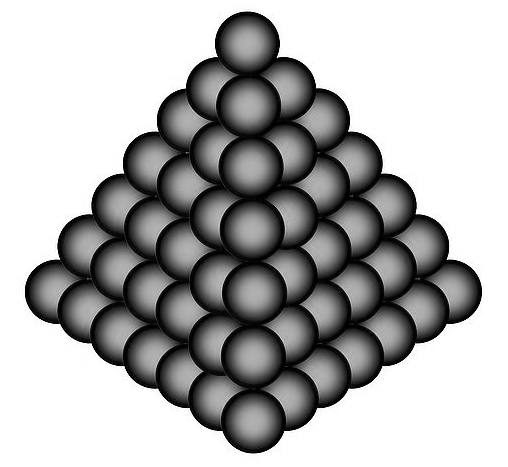
The problem of packing objects is very old and its history goes back to Antiquity (see for example the magnificent monograph [2]). One of the most famous packing problems is known as the Kepler problem, which consists of placing equal balls so that there is the least amount of free space between them. This problem was proposed to Kepler by Sir Walter Raleigh’s assistant, Thomas Harriot, in the early 17th century. Harriot specifically wanted to know if it was possible to prove that the best way to stack cannonballs was precisely the one that had been used since time immemorial: a pyramidal structure of balls (also known as face-centered cubic packing) like the one shown in the figure below:

Kepler tried to solve the problem proposed by Harriot but could not find any proof, although he does mention the problem in his book The Six-Cornered Snowflake, published in 1611 and considered today the foundational book of crystallography, and suggests that the best way to stack balls is in a pyramidal shape.

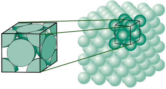
In order to determine the best way to pack the balls, the concept of density of a packing is needed, which is simply the fraction of space contained by the spheres. The following figure shows the procedure to be carried out to calculate this density in the case of face-centered cubic packing, which consists of taking an l side cube and calculating the volume of the spheres and fragments of them contained in this cube and dividing it by its volume.

 

The first rigorous demonstration of Kepler’s problem is due to Gauss, who in 1831 proved that there was no better way to place balls on a net (i.e. balls placed in an “orderly” fashion) than that suggested by Kepler and further calculated that the density in that case was \(\pi/\sqrt{18}\approx 0.74048\dots\) But what happens if we do not have to place the balls in an orderly pattern? This situation was much more complicated and constituted one of Hilbert’s famous problems that became known as Kepler’s conjecture. From the mathematical point of view, Kepler’s conjecture is an optimization problem with an infinite number of variables and we already know what happens with infinity. The first relevant step in solving Kepler’s conjecture was taken by the Hungarian mathematician László Fejes Tóth, who in 1953 reduced the problem to one with a finite number of variables and also suggested that it could surely be solved with the help of computers. Fejes Tóth’s idea was to use the so-called Voronoi cells that were already discussed in this blog also in relation with the placement of objects. And so in 1998 Thomas Hales –with the help of computers– and one of his doctoral students Samuel Ferguson proved the famous conjecture (not without some controversy because mathematicians do not like a test made by a machine). For more information see, for example, [3,4].

We are, however, interested in another problem: that of optimally packing circles in the plane. In this case the solution when the circles are on a net is due to Lagrange, who in 1773 proved that the best way to pack circles on the plane is hexagonal packing (as in the honeycombs) which we can see in the following figure:

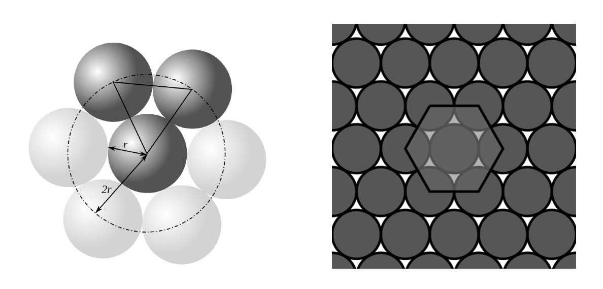
In this case the density is \(\pi/\sqrt{12}\approx 0.9069\ldots\) Once again the question arose as to whether there could be irregular packaging with lower density. The answer is no and the first proof is due to the Norwegian mathematician Axel Thue in 1890, which was generalized in 1940 by the same Hungarian mathematician mentioned above, László Fejes Tóth.

But what if we change the problem to one that is easier to enunciate? For example, what is the best way to pack \(N\) equal circles into a square or a rectangle of given dimensions without them overlapping, so that the radius of the circles is as large as possible. This problem is equivalent to the problem of knowing how many circles we can pack into the square (rectangle) so that the distance between their centres is greater than or equal to a pre-set distance.

This problem is an optimisation problem (geometric) of great interest because of its technological applications (for example, it tells us how to distribute mobile phone repeater antennas) and in our case, because it helps us discover how to optimally distribute the students in a class so that they are all at a distance greater than or equal to a certain pre-fixed distance.

This optimization problem is quite complicated and is still far from being solved in a general form. In fact, unlike the case of a square, where the optimal analytical solutions for a certain number of circles are known, the case of a rectangle is practically unknown.

What is interesting is that there are tremendously efficient numerical algorithms that allow us to find the optimal distributions for not very large \(N\) values. In this work we are going to use the results obtained by E. Specht [5] and that are freely accessible from his website (where a program for the calculation of the distribution in a square is also included).

Before solving our back-to-school problem we are going to consider the question of how to place a certain number of circles in a square of side 1 (this one is the unit that suits us, for example one meter, 7 meters, etc.). In the figure below we have placed 25, 26 and 27 circles respectively inside a square so that they do not overlap and that the minimum distance between their centres is as large as possible.

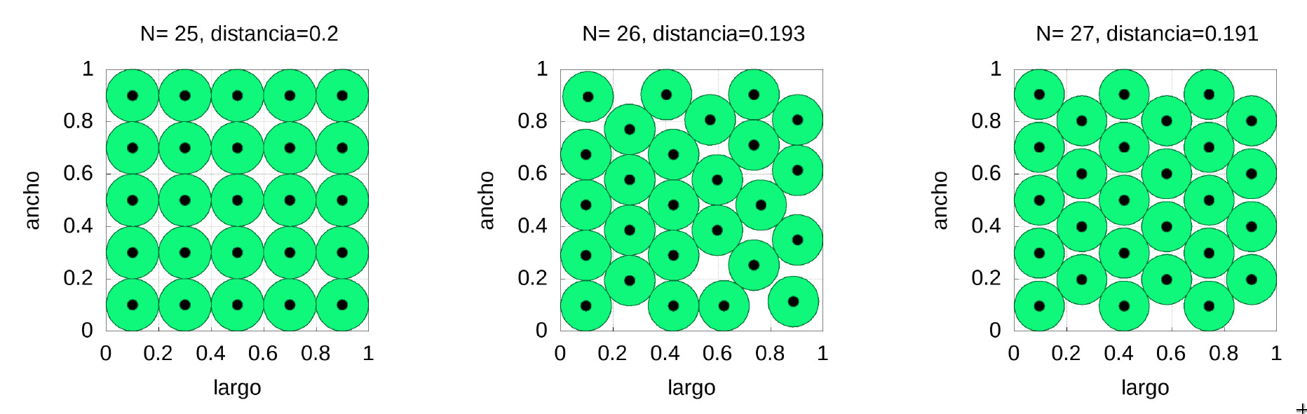
In the figure above we can also see the enormous difference in distribution when placing an extra ball. Above each figure we see the minimum distance between the centres. Note that there is almost no difference on minimum distances (barely \(4.5\%\) between the 25 and 27 circles configurations), but there is a huge difference in the shape of the distribution, with the 26 circles being much more complicated to implement in practice (if we think of a real classroom we would have to immobilise the desks). It should also be noted that in the case of 25 circles we have a distribution similar to that of simple cubic packaging, while in the case of 27 it is very similar to the optimal pyramidal packaging (both in their 2D version).

But let us now imagine that what we want is not to distribute the circles, but their centres (which is what would really be interesting if we are thinking of students and classrooms) in such a way that between them there is a distance greater than or equal to \(d\). It is clear that in this case none of the previous distributions is optimal because the centres can coincide with the sides of the square as shown in the following figure, and it is also obvious that the total number of centres is going to increase with respect to the case discussed above. To solve this, we can simply enlarge the side of our square by the required distance \(d\) rand then conveniently move the distribution obtained. Let us take as an example the case of 25 circles. If we enlarge the side of the square by the fixed distance \(d=0.2\) the result now is that we can place 36 circles. If we move the distribution to the left a distance \(d/2\) and down a distance \(d/2\) we obtain the distribution of the centres shown in the following picture (right).

Using the previous procedure we can see how the centres of 36, 37 and 39 circles would be distributed

Clearly, it is much easier to implement any of the 36 or 39 centre distributions than the 37 centre distribution.

What if what we have is a rectangle? It is clear that in this case an extra parameter must be taken into account: the ratio between width and length. Let’s denote this quotient with the letter \(c\), so if \(l\) is the longest side of the rectangle its shortest side (width) will be \(c\cdot l\). Let’s show two examples.

For the case \(c=0.7\) and requiring that the minimum distance between spheres be \(0.2\) we have that the maximum number of circles is 16, but their distribution is hard to implement in practice. However, 18 circles can be distributed much more easily and the distance hardly differs, as shown in the following figure:

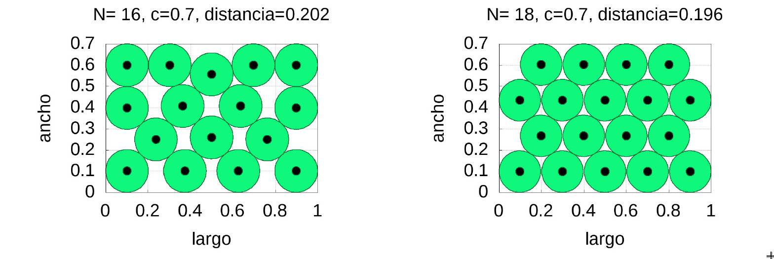
As a curiosity we have to say that the density of the packing of 16 circles is \(0.7303\) while that of the 18 circles is \(0.7745\), 4% higher.

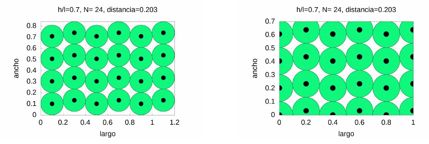
If our interest is to distribute the centres in the rectangles, the problem is much more complicated than in the case of the square, as the sides are unequal. Since we only have the positions of the centres and optimum radii, the procedure described for the case of squares (increasing the side and then moving the rectangle) may not lead us to the optimum solution, although for the number of circles we are using (less than 40) it is almost certain that it will not differ much. In the following figure we show the enlarged rectangle (left) and the final result (right):

Something similar happens if we take \(c=0.8\). If the reader is interested, he can try it himself (the program made with Maxima CAS to prepare this work is available to all those interested from the authors’website). We will end up showing how we can distribute the students in the classrooms.

“Packing” the students in the classrooms.

As an example we are going to show how students should be distributed in a classroom so that they are at a distance greater than or equal to \(1.5\) metres, which is the distance recommended by the health authorities. Our goal is to find the optimal distribution so that the effective area of the class can be used to its fullest, i.e. that as many students as possible enter the class. Let’s show two representative examples.

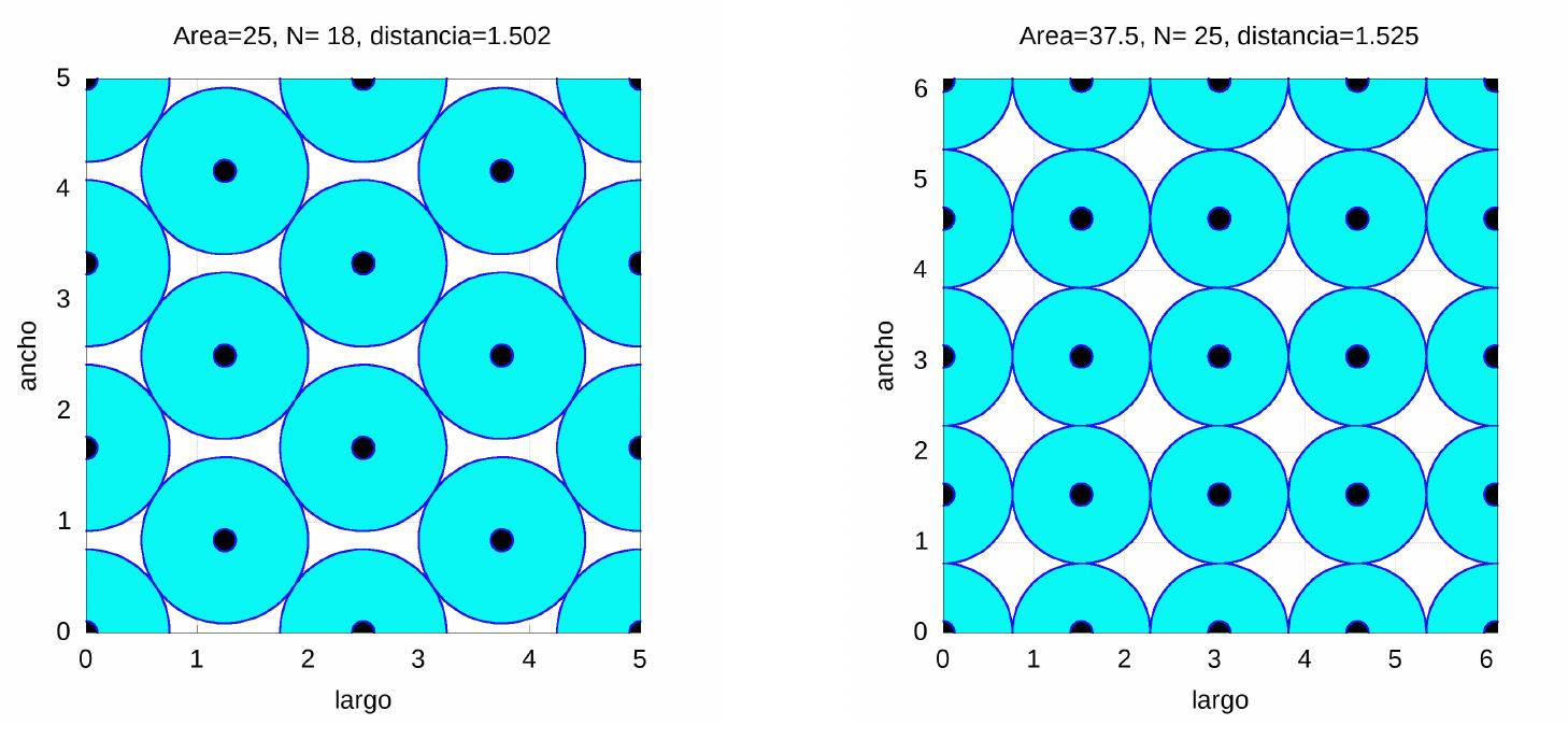
We start with a square 50 square meters classroom and a \(37.5\) sqm square classroom. These numbers are not chosen at random. According to current legislation (Royal Decree 132/2010, of 12 February, which establishes the minimum requirements for centres that teach the second cycle of infant education, primary education and secondary education), an infant classroom must have at least 2 square metres per school post and a maximum of 25 students per school unit and a primary classroom must have \(1.5\) square metres per student and a maximum of 25 students. In the case of secondary and high school, they are also \(1.5\) square metres per student with a maximum of 30 and 35 students respectively (which gives 45 and 52.5 square metres respectively).

In our calculations we will assume an effective area of 50 and 37.5 square meters, respectively (which implies a much larger than average classroom). Let’s imagine this ideal classroom that many media talk about of 50 square meters. Ideally we could place 32 students, but the distribution is quite capricious, so it is much easier to reduce the number of students to 30 which leads to a distribution almost equal to that of the hexagonal packing we have already mentioned. In the following figure we show both distributions:

In the case of a primary classroom with 37.5 useful square meters, up to 25 students can be placed (in a distribution similar to that of simple cubic packaging), while in the case of a 25 square meter classroom, something much closer to reality (several schools in Seville have classrooms with areas no larger than this), 18 can be distributed with a distribution very similar to the hexagonal one.

Finally, as a curiosity we show the results for \(37.5\) and \(50\) sqm classrooms whose ratio \(c\) between width and length is \(c=0.7\).

Conclusions

Considering all the above, we can conclude that the number of students that should be accepted in the classrooms depends (which is obvious) not only on the useful area available, but also on its shape. The optimal solution as we have seen is not necessarily the easiest to apply in practice as one has to take into account not only the safety distance but also the exact position where the desk has to be placed.

To conclude, it is worth noting the following important issues:

1. The students are not points so if we want the real minimum distance between students to be closer to the value established by the health authorities of \(1.5\) metres, and assuming that the diameter of the head is about 20 cm, we should have used a distance of \(1.6\) metres in our calculations (so from the centre of the head to the nose of the closest student there will be \(1.5\) metres), that is, increasing the safety distance by about 10 centimetres, which would further reduce the number of students per class.

2. In our calculations we are keeping in mind the effective area, that is, when we have taken for example an area of 50 square meters, that does not mean that the classroom is 50 square meters, but that the effective area where the students can be distributed is that amount. In a real classroom there is, at least, a table for the teacher (in the primary and infant classrooms there are also shelves and more furniture), doors, and a wall with a blackboard. In other words, in a real classroom of 50 square meters (measured from wall to wall) the students cannot be placed on the blackboard wall or on the entrance and exit doors. We have also assumed that the school positions are individual. This is important when talking about overall ratios. It is obvious that the number of students in a class will depend on the size of the class, so these ratios cannot be fixed in a general way, they have to be flexible as they will depend very much on the facilities of each school or high school.

3. Here we have only concerned ourselves with distributing the students in the classroom so that there is a minimum distance between them of\(1.5\) metres. Whether this is enough to avoid contagion is something we cannot know at present. What is clear is that the more people there are in a closed room, in case there are any sick people, the more likely they are to be infected. So a good policy would be to try to relieve classroom congestion as much as possible. One way to do this is for families who prefer to do so to be able to opt for guided online teaching from their school (this is being done in some US areas, or in Russia, for example). There is no such thing as zero risk, but much can be minimised by taking measures such as those mentioned above.

Note from the authors: The program made with Maxima CAS can be downloaded from the authors’ website. Apart from the figures presented here with this program, it is also possible to obtain the arrays with the coordinates where the corresponding school positions should be placed.

References:

[1]  World Health Organization (WHO), Transmission of SARS-CoV-2: implications for infection prevention precautions. Scientific Brief, 9 July 2020 (WHO reference number: WHO/2019-nCoV/Sci\_Brief/Transmission\_modes/2020.3)

[2] P.G. Szabo, M.Cs. Markót, T. Csendes, E. Specht, L.G. Casado, I. García. New approaches to circle packing in a square (with program codes). Springer, (2007).

[3] T.C. Hales, Cannonballs and Honeycombs. Notices AMS, 47 (2000) 440-449. T.C. Hales, An overview of the Kepler conjecture. arXiv:math/9811071 (publicado como Historical Overview of the Kepler Conjecture,  Discrete and Computational Geometry, 36 (2006) 5-20)

[4] P.J. Miana y N. Romero, La historia de la conjetura de Kepler. Contribuciones científicas en honor de Mirian Andrés Gómez. Servicio de Publicaciones de la Universidad de la Rioja, (2010) 367-374.

[5] E. Specht, High density packings of equal circles in rectangles with variable aspect ratio, Comput. Oper. Res. 40 (2013), 58-69.