Introduction
This article is a continuation of a previous post in which we studied the evolution of an epidemic using a very simple toy model (for more details as well as a general discussion on how to build biological models, see that post).
Again, the idea is to take as a starting point a model with four agents involved: the population susceptible to the disease, the infected who are those who have contracted the disease and are able to transmit it, the recovered who are those infected who have recovered from the disease caused by the virus, and finally those who have died from the disease. Again we denote by \(S(t)\), \(I(t)\), \(R(t)\) and \(F(t)\) the number of susceptibles, infected, recovered and deceased, respectively.
In that entry we focused on showing the consequences of containment on epidemic dynamics. In this entry we will try to model how population behaviour and the influence of the media affect the epidemic dynamics.
Description of the model
We will again use the modified SIR model already used in the previous post, which is described by the following system of ordinary differential equations (ODEs)
$$
\frac{dS}{dt} = -\alpha \frac{S I}N + \delta R, \qquad \,
\frac{dI}{dt} = \alpha \frac{ S I}N – \beta I, \qquad \,
\frac{dR}{dt} = \beta I – \delta R,
$$
where N is the total number of people who constitute the population to be studied and which, as can be seen from the equations, is constant and equal to \(N(t)=S(0)+I(0)+R(0)\).
We will treat deaths separately, assuming, as in that entry, that they are a proportion of those infected, \(F(t) = \gamma I(t)\), so that the more infected there are, the greater the number of deaths (whether directly caused or as a consequence of the collapse of the health system). To measure the impact of the epidemic we will use the magnitude \(M_F\) defined by
$$
M_F := \frac{1}{L}\sum_{n=1}^L v_n, \qquad \qquad \qquad \qquad (M)
$$
where \(L\) is the number of components of the vector \(V_F\), which is the vector resulting from the numerical simulation to solve the ODE system of the model between times \([t_1,t_2]\).
The novelty consists of generalising the coefficient \(\alpha\) (rate of infectious contacts between the infected and the susceptible). To do so, we introduce the concepts of public perception of risk and intensity of public response to that perception. As a starting point we will take the idea introduced in [1] and used, for example, in this post. So, we will introduce the function \(\psi_{\alpha}\), that generalize the previously introduced function \(\alpha(t)\)
$$\psi_\alpha(t,D) := \alpha(t) \left[1-c\, \phi\left(\frac{D(t)}{N(t)}\right)\right]^{\kappa},$$
where \(\phi\) is some function dependent on the public sense of risk \(D\), and \(N\) is, as before, the total number of individuals in the population.
For simplicity (and following an idea similar to the one developed earlier in this post) we will take \(D(t)=I(t)\). The reason is that in our model we have assumed that the number of deaths caused by the epidemic (directly or indirectly) as well as the number of severe cases are proportional to the number of infected people, so the higher the number of infected people, the higher this number will be and, therefore, the population would realise the risk of contracting the disease and should behave more responsibly. Finally, \(c\in[0,1]\) is a certain constant (fixed beforehand or estimated as appropriate) so that \(|c \phi\left({D(t)}/{N(t)}\right)|<1\) regardless of the time instant we consider.
The function \(\phi\) must be a function that fulfils a minimum of properties. For example, it must be increasing in its variable since, as the sensation of risk increases, its value must increase so that \(|1-c\phi(x)|<1\) is smaller since, as we have already mentioned, if there is a greater perception of risk, the behaviour of the population will be more responsible and therefore \(\psi_{\alpha}\) will be smaller.
Finally, we will introduce the exponent \(\kappa\geq0\) which tries to model the intensity of the population’s response. In our case, we will relate it to the message of the political-health authorities distributed by the media. If the authorities maintain a narrative that explains the risks and consequences of contracting the disease and urges the population to follow the health regulations, \(\kappa\) will take large values so that \(\psi_\alpha(t,D)\) will be even smaller, while if they transmit an overly optimistic message, \(\kappa\) will take small values and \(\psi_\alpha(t,D)\) will increase compared to the previous case. That is, \(\kappa\) will act as an amplifying factor. It is important to note that although in [1] it is assumed that \(\kappa\) is constant over time, this value could well vary depending on the perception of risk (e.g. if over the course of the epidemic management there is a change in the attitude of authorities and the media).
In this entry we will use two different \(\phi_i : [0,1] \to [0,1]\) functions. One will be the following step function
$$ \phi_1(x) = \left\{ \begin{array}{ll} v_1, & \mathrm{if\ } x \in V_1, \\ v_2, & \mathrm{if\ } x \in V_2, \\
v_3, & \mathrm{if\ } x \in V_3,\\
v_4, & \mathrm{if\ } x \in V_4,\\
\end{array} \right.
$$
where \(v_i\in[0,1]\) and \(V_i\) are disjoint and connected sets such that their union is the interval \([0,1]\), which models a risk perception that jumps as contagions increase until it reaches a maximum value. The second function \(\phi_2\) that we will use will be
$$ \phi_2(x) = x, $$
and models a situation where risk perception increases as contagion increases in a linear fashion. Note that in the second case, the function \(\psi_{\alpha}\) is of the form
$$ \psi_\alpha(t,D) := \alpha(t) \left[1-c\, \frac{I(t)}{N(t)}\right]^{\kappa}, $$
which coincides with the one used in this already mentioned post. It is obvious that we could also use a step function up to a value of the quotient \(I/N\) and then a linear one, among many others.
In the following figure we will show the graphs of both functions:
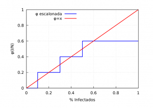
Thus, the equations to take into account the behaviour of the population will be:
$$
\frac{dS}{dt} = – \psi_{\alpha} \frac{S I}N + \delta R, \quad \,
\frac{dI}{dt} = \psi_{\alpha} \frac{ S I}N – \beta I, \quad \,
\frac{dR}{dt} = \beta I – \delta R.
$$
Simulations
Let’s look at some numerical examples to see how population behaviour affects epidemic dynamics. We will use the following values for the numerical coefficients of the model: \(\alpha=0.065\), \(\beta=0.03\), \(\delta=0.02\), \(\gamma=0.002\), as well as the initial conditions \(s(0)=10000\), \(i(0)=100\) and \(r(0)=0\). For \(c\) we will use the value \(c=0.01\). It is clear that if \(\kappa=0\) we recover the equations of the basic model.
Throughout this section we will use the following function \(\phi_1\).
$$
\phi_1(x) = \left\{
\begin{array}{ll}
0, & \mathrm{if\ } x \in [0, 0.1], \\
1/5, & \mathrm{if\ } x \in (0.1, 0.3], \\
2/5, & \mathrm{if\ } x \in (0.3, 0.5],\\
3/5, & \mathrm{if\ } x \in (0.5, 1].\\
\end{array} \right.
$$
Furthermore, in all the cases to be studied we will calculate the magnitude \(M_F\) in the interval \([0,500]\) in such a way that the maximum of the corresponding wave is included.
Case when \(\phi\) is a step function
We will begin by analysing the case when \(\phi\) is the step function above. In general we will distinguish three cases.
1. when the population has an irresponsible behaviour where \(\kappa=0\) (we act as if the epidemic is already over influenced by irresponsible narrative by the authorities and the press),
2. when the behaviour is moderate \(\kappa=100\) (the population relaxes and neglects many of the health measures influenced by an unclear discourse by the authorities), and
3. responsible behaviour \(\kappa=200\) influenced by a coherent and cautious approach of the authorities and the media recommending and explaining the health measures to be complied with.
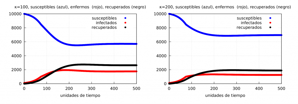
The following graphs show the results of the numerical simulation for the moderate and responsible response cases (the irresponsible case corresponds to the initial model we saw earlier). On the left is the evolution of the epidemic using \(\phi_1\) and \(\kappa=100\), and on the right the case when \(\kappa=200\).
It is useful to represent in the same graph the evolution of the three cases considered.
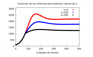
In the graph above we can observe the evolution of the infected using \(\phi_1\). In red we represent the case \(\kappa=0\) with \(M_f^{\kappa=0} = 1922\), in blue \(\kappa=100\) with \(M_f^{\kappa=100} = 1557\), in black \(\kappa=200\) with \(M_f^{\kappa=200} = 1141\). As can be seen, \(M_F\) decreases significantly if the message from the authorities makes the population behave more responsibly.
Case when \(\phi\) is the linear function
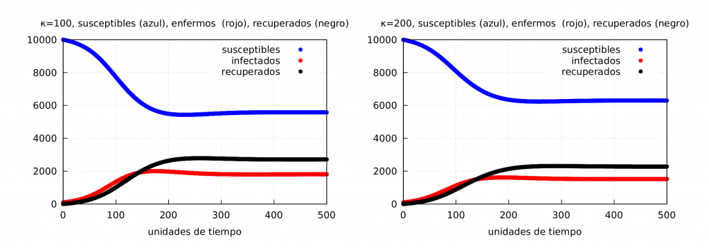
Below we show the graphs corresponding to the case when \(\phi\) varies linearly. On the left we show the evolution of the epidemic using \(\phi_2\) with \(\kappa=100\) and on the right with \(\kappa=200\).
In the following graph we can compare the curves of the evolution of the infected using \(\phi_2\). In red we represent the case when \(\kappa=0\) with \(M_f^{\kappa=0} = 1922\), in blue \(\kappa=100\) with \(M_f^{\kappa=100} = 1581\), and in black \(\kappa=200\) with \(M_f^{\kappa=200} = 1322\).
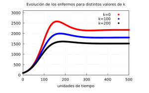
As shown in this last graph, again the value of \(M_F\) decreases significantly if the message from the authorities manages to convey the need for more responsible behaviour.
It should be noted that, in general, there is no great difference when simulating the evolution of the epidemic using either of these two \(\phi\) functions as long as the \(I/N\) ratio is not too close to 1. In the latter case, the \(\phi_2\) function values practically one, while \(\phi_1\) from a certain critical value of \(I/N\) takes the same value (which in our numerical example is \(I/N=1/2\)).
Case when the \(\kappa\) factor is dynamic
Let’s see what happens if we use a linear \(\phi\) but make \(\kappa\) time-varying. Given that \(\kappa\) acts as an amplifier of the population’s sense of risk, we will assume that it is proportional to the number of infected people, i.e. as \(I\) increases, the population reacts more responsibly and this good behaviour is amplified by a stronger message from the political and health authorities about the importance of maintaining this good behaviour. We will take the proportionality factor to be equal to \(1/10\) so that \(\kappa\) will take at most a value less than one tenth of the maximum reached with the basic model (which is about 250). The results are shown in the graph below:
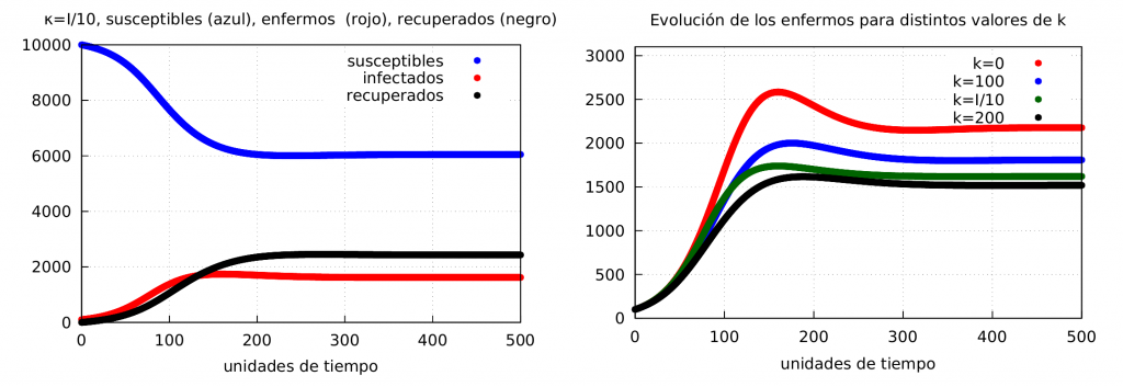
Thus, in the left graph we show the evolution of the epidemic using \(\phi_2\) and with \(\kappa\) dynamic. On the right, the comparison of the evolution of the infected using \(\phi_2\), in red when \(\kappa=0\) with \(M_f^{\kappa=0} = 1922\), in blue \(\kappa=100\) with \(M_f^{\kappa=100} = 1581\), in black \(\kappa=200\) with \(M_f^{\kappa=200} = 1322\) and in green \(\kappa=I/10\) with \(M_f = 1431\).
Case when \(\phi\) is the linear function and a confinement is applied
Finally, let’s see what happens if the authorities decide to apply containment and the behaviour of the population is taken into account. We will focus on the case \(\kappa=200\) since the decision by the authorities to apply containment implies (or should) that the message is a high risk of infection so the population will necessarily be much more cautious than in a case without containment. In this case we will apply a confinement equal to the one used in the previous entry (see the formula for \(\alpha(t)\)) with the parameters \(\alpha_1 = 0.065\), \(\alpha_2 = 0.05\), \(t_i = 150\), \(\tau = 50\)). The results can be seen in the following graph:
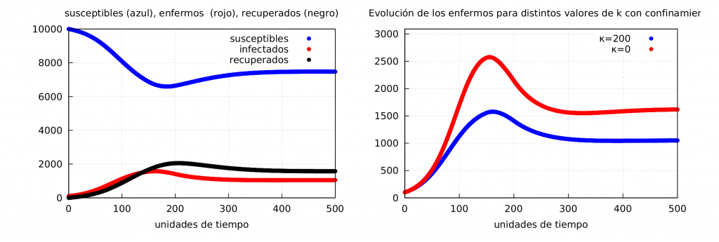
On the left we show the evolution of the epidemic using \(\psi_2\) with \(\kappa=200\) and confinement. On the right we show how the infected evolve using \(\psi_2\) and permanent confinement with \(\kappa=200\) (blue) with \(M_f^{\kappa=200} = 1050\) and \(\kappa=0\) (red) with \(M_f^{\kappa=0} = 1579\).
Needless to say, it is much more effective if confinement is coupled with responsible behaviour of the population amplified by a coherent narrative from the authorities (rigorously conveyed by the media) about the risks of contracting the disease and the importance of following the corresponding health regulations, as shown in the graph on the right of the figure above and reflected in a lower value of the magnitude \(M_F\) used to measure the severity of the epidemic (in particular, a higher value will imply a higher mortality).
Conclusions
In this entry we have tried to include in our toy model the effect of individuals’ behaviour on the dynamics of an epidemic. To introduce this behaviour into our model we have used a \(\phi\) function that quantifies the public feeling of risk, a concept discussed in several previous works. This behaviour will be amplified by the message of the authorities and the media through an amplifying factor \(\kappa\) so that we will have a generalisation of the rate of infectious contacts \(\alpha\) that takes into account not only the possible measures taken by the different governments (such as confinements) but also the behaviour of the individuals in the population itself.
Given the examples given in this section, we can conclude that our behaviour in the face of an epidemic (in particular during the pandemic in which we are involved) can greatly reduce the number of infected people and with it the demographic and economic consequences that this brings. Social behaviour can lower the infection rate, making confinement unnecessary.
Our perception of the risk together with a successful communication policy by the authorities and the media in order to make us aware of the risk and act accordingly (in our model this translates into an increase in the value of \(\kappa\)) can significantly reduce the negative effects of the epidemic (measured by the magnitude \(M_F\)) without the need for strict containment. As we have seen, misinformation or the relaxation of the population (a small \(\kappa\)) only increases the rate of contagion, increasing the number of infected people.
Finally, it should be noted that in the worst-case scenario, the application of containment together with good behaviour of the population is the best way to control an epidemic.
All of the above should be borne in mind by the public, the authorities, and the media at a time when infections are on the rise again, and when news from other countries, such as the USA, is not at all flattering about the increase in infections, even in vaccinated people. Good behaviour is essential to prevent infection, resulting in lower mortality and hospital pressure.
Bibliography
[1] D. He, J. Dushoff, T. Day, J. Ma, D.J. Earn, Inferring the causes of the three waves of the 1918 influenza pandemic in England and Wales. Proc. R. Soc. B: Biol Sci. 280, (2013), 20131345 https://dx.doi.org/10.1098/rspb.2013.1345
To learn more about epidemic modelling:
M. J. Keeling, P. Rohani, Modeling Infectious Diseases in Humans and Animals, Princeton University Press, Princeton, 2007.

Leave a Reply