In this third post focused on how an epidemic can be modelled (the previous posts can be seen here and here) we will show two possible models to describe the dynamics of the epidemic when a vaccine against it is available. The first is a very simple modification of our basic model described in the first post and for which the equations are
$$ \dfrac{dS}{dt} = -\alpha \frac{S I}N + \delta R, \qquad \, \frac{dI}{dt} = \alpha \frac{ S I}N – \beta I, \qquad \, \frac{dR}{dt} = \beta I – \delta R, \qquad (*)$$
while the second, although simple, is somewhat more complex as it will include two new populations: the vaccinated and the vaccinated infected.
Modifying the base model
Comenzaremos con el primero de los modelos que describiremos en tres pasos:
I: Decrease in the infection rate \(\alpha\). The idea is that, as a result of vaccination, the infection function \(\alpha(t)\) will vary from an initial value \(\alpha_0\), which is the value we would have without vaccination, to a value \(\alpha_1\), which is the infection rate in the case where all individuals would be vaccinated. This case is similar to the model used for lockdown (see the first post) only with a different \(\alpha(t)\) function. Hereafter we will denote by \(t_v\) the time instant when vaccination of the population begins. Our interest is to see what happens for times longer than \(t_v\). Thus, we propose the following step function:
$$
\alpha(t) := \begin{cases}
\alpha_0, & t \leq t_v, \\
\max\left(\dfrac{\alpha_1-\alpha_0}{\nu}(t-t_v)+\alpha_0, \alpha_1\right), & t > t_v,
\end{cases}
$$
where \(\alpha_1 < \alpha_0\).
II: Increase in the recovery rate \(\beta\). The idea in this case is that, after vaccination, the value of the recovery rate is higher than before vaccination, so the function \(\beta(t)\) will vary from a value \(\beta_0\) which is the initial state without vaccination, to a value \(\beta_1>\beta_0\) which would be the recovery rate in the case when all individuals are vaccinated. Unlike the confinement model, where the recovery rate is constant, we will assume that vaccination not only decreases infection, but also increases the recovery rate. As before, \(t_v\) will indicate the point in time when vaccination is started. Thus, we propose the following step function
$$
\beta(t) :=
\begin{cases}
\beta_0, & t \leq t_v, \\
\min\left(\dfrac{\beta_1-\beta_0}{\nu}(t-t_v)+\beta_0, \beta_1\right), & t > t_v,
\end{cases}
$$
III: Mixed model. Given that the vaccine is expected to modify both the \(\alpha\) and \(\beta\) parameters, the most reasonable way to show how vaccination changes the dynamics of the epidemic is to combine both models to obtain a mixed model where, if vaccination is effective, we would see a decrease in the infection rate \(\alpha\) and an increase in the recovery rate \(\beta\). This leads us to propose the following model, whose equations are very similar to those of the basic model (*):
$$
\frac{dS}{dt} = -\alpha(t) \frac{S I}N + \delta R, \qquad \,
\frac{dI}{dt} = \alpha(t) \frac{ S I}N – \beta(t) I, \qquad \,
\frac{dR}{dt} = \beta(t) I – \delta R,
$$
where now \(\alpha\) and \(\beta\) are the functions defined in points I and II, respectively.
From the analysis carried out in the first post, it follows that, if \(\alpha_1<\beta_1\), then vaccination would end the epidemic. Otherwise, the epidemic would persist, although the vaccine could drastically reduce the value of the coefficient \(\gamma\), associated as we have already seen with the percentage of those infected who die or are seriously affected by the disease.
Simulations of the Simplified Vaccination Model
Let’s look at some examples showing both possibilities of what would happen if a preventive vaccine is started some time after the epidemic appears.
In the first case, we will assume that we do indeed have a good enough vaccine that lowers the infection rate and increases the recovery rate by a considerable amount. Let us then look at the difference in the number of infected people between having a vaccine and not having a vaccine. In all cases we will take the values \(\alpha_0=0.065, \beta_0=0.03, \delta=0.02, \nu=400, t_v=200\) and vary the other values, which will allow us to compare the number of infected with those of the base model (*).
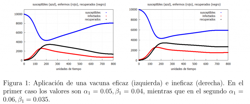
If we compare the graph on the left in figure 1 with that of the basic model (see the first post) podemos ver una notable diferencia entre el número de infectados, siendo la vacunación de la población una de las herramientas más eficaces para salvar vidas, siempre y cuando la vacuna sea realmente eficaz. Hemos de señalar que en el ejemplo considerado la vacunación no acaba con la epidemia puesto que \(\alpha_1>\beta_1\).
Suppose we suspect that the vaccine does not work, one way to see if this is true would be to look at the evolution of those infected (remember that in the base model (*) the number of deaths was proportional to the number of infected) when no vaccine was available and compare it with the evolution of those infected when the vaccine is available. If our suspicions were true then we should see a graph like the one on the right of figure 1, which is very similar to the one that would be obtained with the base model (*), since the difference in the number of infected is not significant, i.e. the vaccine has not performed its expected function very well.
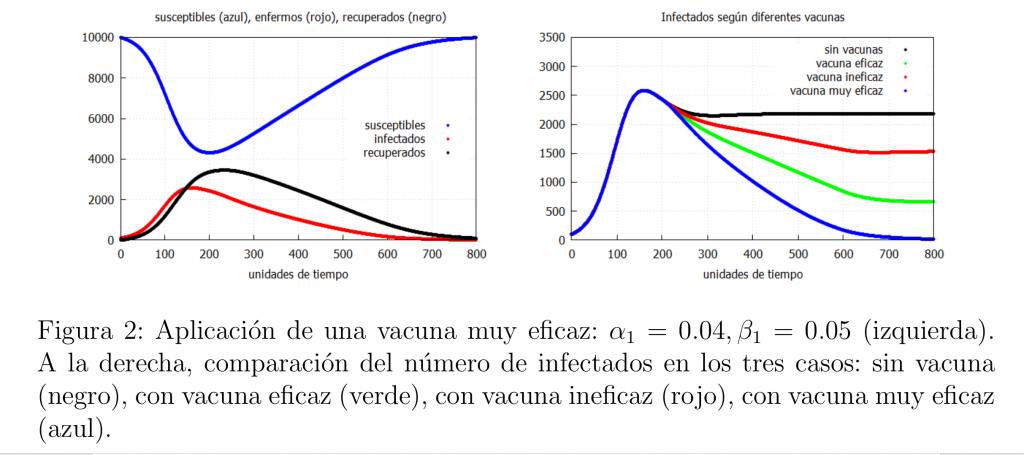
Let us note that if we get a really effective vaccine, i.e., such that \(\alpha_1<\beta_1\), then we can end the epidemic. An example of such a vaccine is that of smallpox, which caused its global eradication in the 1980s. Thus, we would have the behaviour shown in the graph on the left of figure 2. Finally, in figure 2 on the right we show a graph with the evolution of the infected in the cases analysed in this case.
SIRVI model
The above model is certainly too simple, as it is obvious that the epidemic dynamics in the vaccinated population will be generally different from those in the unvaccinated population. We will therefore consider a slightly more complex model that takes this difference into account, which will consist of including two new sets of individuals in the population: those who are vaccinated and those who, while vaccinated, may become infected with the disease. This new model should help us to better understand the dynamics of the epidemic by taking into account the difference (advantage) of being vaccinated.
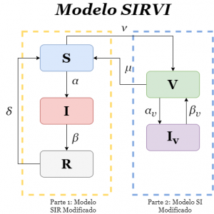
The idea of this model is based on merging two models: on the one hand the modified SIR model (*) and a modified SI model that will be used to describe the interaction between the vaccinated population and those who are still vaccinated but become infected. The interactions within the SIR model are the same as those we have already used. We will call this model the SIRVI model.
The new interactions in the model start when the vaccine comes into play. Thus, we will define the rate of vaccination of the population which we will denote by \(\nu\), this being the link between the susceptible and the vaccinated. We will also have a link in the opposite direction, we will call the rate of loss of immunity of the vaccinated \(\mu\). The existence of a \(\mu\neq0\) could be due to the emergence of mutations in the disease-causing virus for which the vaccine applied would not be effective or, simply, that the vaccine does not work in 100% of the cases. On the other hand, we are going to assume that the vaccinated population can also catch the disease but, thanks to the vaccine, their infection rate will be lower (as well as the percentage of deaths while vaccinated) and their recovery rate will be higher than the unvaccinated, which translates into an infection rate for vaccinated people \(\alpha_v\) and a recovery rate for vaccinated people \(\beta_v\). Schematically, the model will be as follows:
\begin{equation*}
\left\{\begin{split}
\frac{dS}{dt} = & -\alpha \frac{S (I+I_v)}N + \delta R-\nu+\mu V, \\
\frac{dI}{dt} = & \alpha \frac{ S (I+I_v)}N – \beta I, \\
\frac{dR}{dt} = & \beta I – \delta R, \\
\frac{dV}{dt} = & -\alpha_v \frac{V (I+I_v)}N + \nu -\mu V +\beta_v I_v, \\
\frac{dI_v}{dt} = & \alpha_v \frac{ V (I+I_v)}N-\beta_v I_v.
\end{split}\right. \qquad (**)
\end{equation*}
Here, \(\alpha\) and \(\alpha_v\) are the infection rates, \(\beta\) and \(\beta_v\), the recovery rates, and \(\nu\), the rate at which vaccination of the population progresses, where the subscript \(v\) indicates the rates of the vaccinated population. \(\mu\) is a rate that indicates how much of the vaccinated population becomes susceptible again (due to various causes such as a mutation of the virus reducing the effectiveness of the vaccine or loss of immunity over time). If \(\mu = 0\) we would be in the case where, after vaccination, individuals do not lose immunity and therefore the vaccine is 100% effective. Note that
$$
\frac{dS}{dt} +\frac{dI}{dt} +\frac{dR}{dt} +\frac{dV}{dt} +\frac{dI_v}{dt}=0,
$$
i.e. the total number of individuals in the population \(N=S(t)+I(t)+R(t)+V(t)+I_v(t)\) is constant.
The stationary solutions of the system (**) are as follows:
\begin{equation*}
S_1=N-\frac{\nu}{\mu},\quad
I_1=0,\quad
R_1=0,\quad V_1=\frac{\nu}{\mu},\quad {I_v}_1=0,\quad (sol 1)
\end{equation*}
and
\begin{equation*}
\begin{split}
S_2= & -\frac{\beta \left( {{\alpha}_v} \nu-N {{\beta}_v} \mu\right) }{\alpha {{\beta}_v} \mu},\quad\\
I_2= & -\frac{\delta \left( {{\alpha}_v} \nu-N {{\beta}_v} \mu\right) \left( \alpha {{\beta}_v} \nu-{{\alpha}_v} \beta \nu+N \beta {{\beta}_v} \mu-N \alpha {{\beta}_v} \mu\right) }{\alpha {{\beta}_v} \mu \left( {{\alpha}_v} \beta \nu-N {{\beta}_v} \delta \mu-N \beta {{\beta}_v} \mu\right) },\\
R_2= & -\frac{\beta \left( {{\alpha}_v} \nu-N {{\beta}_v} \mu\right) \left( \alpha {{\beta}_v} \nu-{{\alpha}_v} \beta \nu+N \beta {{\beta}_v} \mu-N \alpha {{\beta}_v} \mu\right) }{\alpha {{\beta}_v} \mu \left( {{\alpha}_v} \beta \nu-N {{\beta}_v} \delta \mu-N \beta {{\beta}_v} \mu\right) }, \\ V_2= & \frac{\nu}{\mu},\\
{I_v}_2= & \frac{{{\alpha}_v} \delta \nu \left( \alpha {{\beta}_v} \nu-{{\alpha}_v} \beta \nu+N \beta {{\beta}_v} \mu-N \alpha {{\beta}_v} \mu\right) }{\alpha {{\beta}_v} \mu \left( {{\alpha}_v} \beta \nu-N {{\beta}_v} \delta \mu-N \beta {{\beta}_v} \mu\right) }, \quad (sol 2)
\end{split}
\end{equation*}
where, in both cases, \(N=S(0)+I(0)+R(0)+V(0)+I_v(0)\).
It should be noted that the first solution (sol 1) corresponds to the case when the epidemic disappears. In the case of the second solution (sol 2) an analysis at first sight is not conclusive given the number of parameters involved. However, it can be seen that under certain assumptions the total number of infected \(I_v + I\) is less or equal to the number of infected \(I_{O}= (\alpha-\beta)\delta N/(\delta+\beta)\alpha\) of the initial model (*), which is to be expected since it is assumed that the vaccine itself does not increase the number of infected.
Simulations
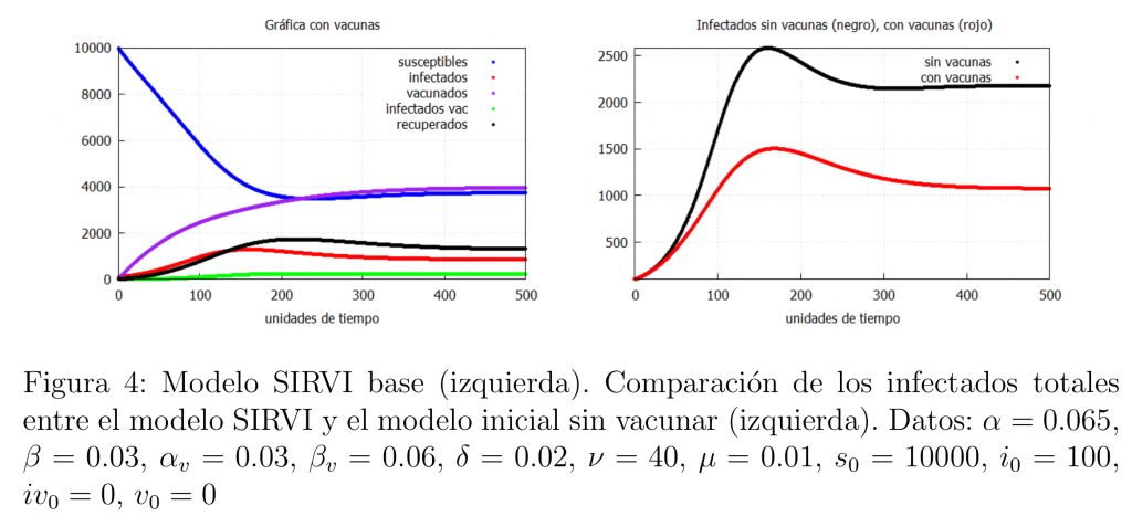
Suppose that with the introduction of the vaccine in the model it works normally, making the vaccinated population more resistant to infection, that is, less infected (\(\alpha\geq \alpha_v\)) and that, if infected, it recovers sooner
(\(\beta\leq \beta_v\)).
In this case we would expect the number of vaccinated infected to be lower than the number of unvaccinated infected and, therefore, that the total number of infected (the sum of unvaccinated and vaccinated infected) is lower than in the basic model (*) (no vaccine). This is what figure 4 shows. In accordance with this, we can see in the graph on the right how the total number of infected with the SIRVI model (\(I+I_v\)) is much lower than those of the SIR model (*). In other words, according to the model, the introduction of the vaccine really helps to reduce the number of infected people, thus reducing the hospital pressure and the number of deaths.
A natural question is how to know if the vaccine is good enough. One option is to vary the \(\mu\) parameter that models the loss of immunity. In fact, a high \(\mu\) indicates that a large number of vaccinees lose immunity and become susceptible. In figure 5 we show what happens if we increase the value of \(\mu\) thus causing the efficacy of the vaccine to decrease.
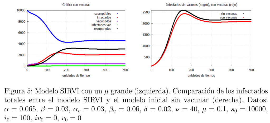
In this case, there is not much difference between vaccination and non-vaccination, i.e. there is not much difference between this case and the basic SIR model (*). This indicates that a rigorous analysis of post-vaccine infectiousness data can help us to know the real efficacy of the vaccine.
We will now look at what happens when the rate of vaccination in the population is very slow. In our model this is equivalent to saying that \(\nu\) is small. The results can be seen in figure 6.
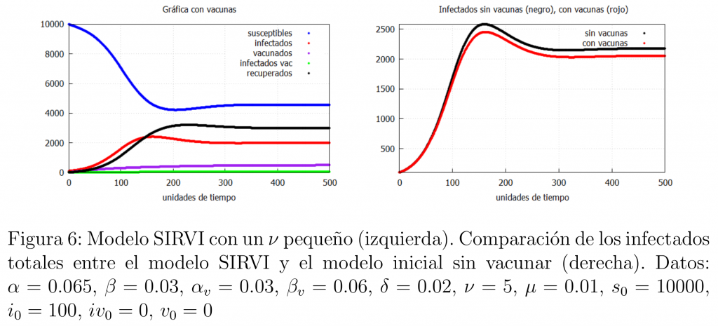
Note that this case is very similar to the case when the vaccine is not very effective. In other words, having an effective vaccine that is not efficiently administered is the same as having an ineffective vaccine. So, if a good enough vaccine is available, the best thing to do, according to our model, is for administrations to ensure that the speed of vaccination is as high as possible and that citizens are vaccinated as soon as possible.
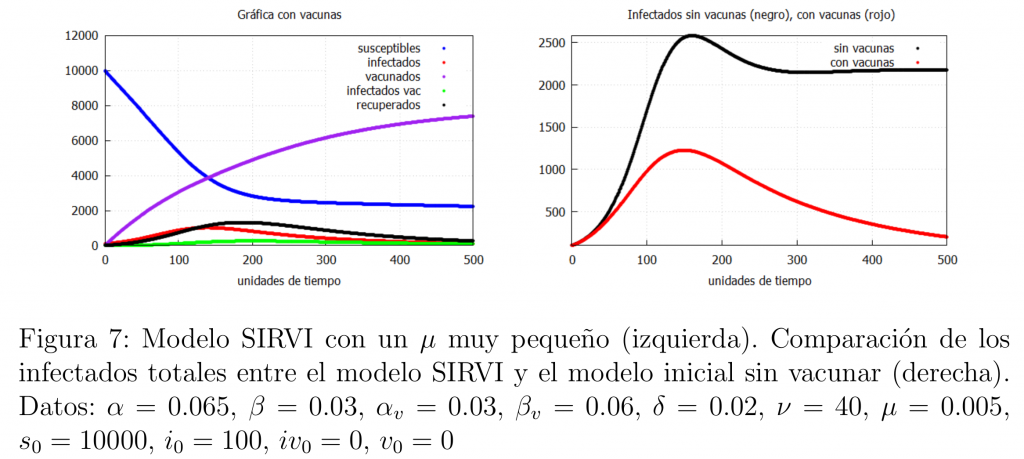
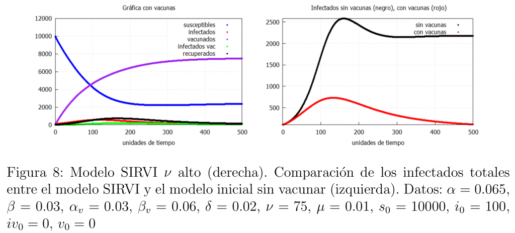
Let us now see what happens when the population is massively vaccinated at a high rate and when we have a vaccine that is extremely good at fighting the virus. In this context vaccination gives us a magnificent tool to end the epidemic. Such an ideal situation can be achieved in two ways:
\(\bullet\) The first case occurs if a highly effective vaccine is available. That is, if the majority of people vaccinated with this vaccine do not lose immunity and show high resistance to the virus. Translated into our model this implies that \(\mu\) takes very small values. The result is shown in figure 7, where we can see how the vaccine manages to end the epidemic.
The second possibility is if the population is mass vaccinated with a high vaccination rate and the vaccine is good enough (even if it is worse than the previous case, i.e., higher \(\mu\)). In this case a similar result is obtained as shown in figure 8.
Conclusions on the use of vaccines
In this post we have shown two models in an attempt to explain how the use of a vaccine can affect the dynamics of an epidemic. In both models, it can be seen that the availability of an effective vaccine helps to reduce the number of people infected and, therefore, reduces both the pressure on hospitals and the number of deaths. One of the main reasons is associated with a decrease in the rate of infection \(\alpha\) and an increase in the rate of recovery \(\beta\).
However, there is a clear difference between the two models, as the second model includes two distinct blocks of populations: those who are vaccinated and those who, even if vaccinated, become infected. This model is somewhat more realistic than the first at the price of making it more complex. In particular, this second SIRVI model allows us to include both the speed of vaccination and the loss of vaccine immunity, both of which are tremendously important variables in ending the epidemic, as we have shown. An obvious conclusion from the model is that a good vaccination rate is as important as a very efficient vaccine.
As a final conclusion we must say that even two models as simple as the ones presented here show that vaccines are undoubtedly a very powerful weapon to fight and eventually end, an epidemic such as the one we are currently involved in. We therefore urge the readers to decide for themselves, after reading this post (and the two previous ones), what is the best way to act in situations as complex as the current covid-19 epidemic.
Learn more about epidemics modelling
N. F. Britton, Essential Mathematical Biology, Springer, London, 2003.
H. W. Hethcote, The Mathematics of Infectious Diseases, SIAM Rev. 42(4), (2000), 599–653.
M. J. Keeling, P. Rohani, Modeling Infectious Diseases in Humans and Animals, Princeton University Press, Princeton, 2007.

Leave a Reply