Alberto Calderón and finding causes from effects (and II)

More about Calderón

This post is the second and last part of another one, dedicated to Alberto Calderón. We will begin with a couple of short anecdotes that affected him, directly or indirectly.

The first of them has as its protagonist one of his professors at the University of Buenos Aires: Julio Rey Pastor. It is said that, in a seminar, he answered a question about the nature of infinity in the following way: “For me, infinity starts at one thousand pesetas”.

The second one has to do with his fondness for tobacco. One day, holding a cigarette in one hand and (how not?) the chalk in the other while he was concentrating on a demonstration in the classroom, he ended up sucking on the chalk, thus unleashing a curious spectacle in front of his students.

(I will not reveal who, but I will tell you that this same incident was once played out by one of our teachers in front of me, around 1980, at a time when we all used to smoke like crazy).

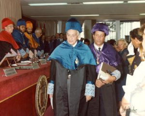
In any case, if we are talking about Calderón, we refer to an exceptional being. He was elected member of the Science Academies of USA, Argentina, Spain, France, Venezuela and Italy and received a considerable collection of scientific awards, including an Honorary Doctorate at Universidad Autónoma de Madrid in 1997.

Uhlmann, Caro and others

Some researchers active in solving Calderon’s problem have been G. Uhlmann, M. Vogelius, J. Sylvester, K. Astala, L. Paivarinta, M. Lassas and P. P. Caro. This will be made clear below.

Let us speak in particular of Uhlmann and Caro.

Guntar Uhlmann, born in 1952, graduated from the University of Chile in Santiago and received his PhD from MIT in Massachusetts (USA).

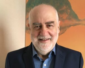
He was later hired at MIT itself, Harvard University, the Courant Institute of Mathematical Sciences, and the Universities of Washington and California. He is currently working at the Institute of Advanced Studies of the Hong Kong University of Science and Technology.

He has been interested in inverse problems for partial differential equations from various points of view. In particular, he has made an important contribution to the solution of the Calderón problem. In some of his recent works, in collaboration with Y. Kurylev and M. Lassas, he has studied inverse problems for nonlinear wave equations and for the Einstein system coupled with scalar field equations. There, the question to be answered is the following:

Can an observer make local measurements to determine the structure of space-time in the largest region where waves can propagate?

The authors respond (a) by reducing the inverse problem to an analogous question where the measurements are “passive”, that is, they do not correspond to choices made by the observer, and then (b) by applying techniques from Lorentzian geometry; see [1-3].

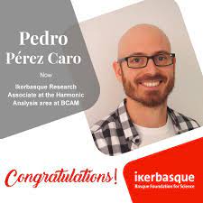
Pedro P. Caro, born in 1982, studied Mathematics at our Faculty and did a Master’s degree at Université P. et M. Curie (Paris 6, France) and a PhD at Universidad Autónoma de Madrid (under the direction of A. Ruiz). He was subsequently hired at the universities of the Basque Country and Helsinki (Finland) and at ICMAT (Madrid). He currently holds a research position (Ikerbasque Research Fellow) at BCAM (Bilbao).

We will see in due course that he has also contributed with significant advances to the resolution of the Calderón problem. In one of his latest works, in collaboration with C. J. Meroño and I. Parissis, he has been interested in what we can call “rotational regularisation”. This is a process that allows to gain regularity through rotation and averaging. The interest in a systematic analysis of it is motivated by the resolution of some inverse problems with non-regular data; see [6].

Learn more (I): The problem and its variants

The electrical impedance tomography problem, also called Calderón’s inverse problem, is as follows: determine the electrical conductivity \(\gamma = \gamma(x)\) of a medium occupying an open set \(\Omega \subset {\bf R}^N\), assuming that we know on the boundary \(\partial\Omega\) for every electric potential (which is arbitrarily imposed) the associated current (which is observed or measured).

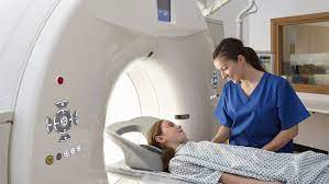
This problem arises when one wants to get a picture of the conductivity or permittivity of some part of the body from measurements on the contour. In practice, conductors are attached to the skin and measurements are made corresponding to small alternating currents applied to the electrodes. The process is usually repeated for a large number of different current configurations. The calculated conductivity provides information on the presence and properties of possible tumours. This technique is considered to be very effective, especially for the early detection of breast cancer; see [4-5].

As mentioned, Calderón formulated this problem motivated by oil prospecting problems. An elastographic variant was presented in this blog, in a previous post. Many others can be formulated, all of them of great interest: evolutionary versions which, as shown in another post, help to describe the evolution of epidemics, versions where the partial differential equation describes the behavior of the temperature of the medium or the wave function of a quantum system, non-scalar problems related (for example) to the determination of a solid inside a fluid, etc.

In an idealised situation, the potential \(u = u(x)\) can be assumed to be the solution to the system

$$
\left\{
\begin{array}{l}
\sum_{i=1}^N \partial_i (\gamma(x) \partial_i u) = 0, \quad x \in \Omega
\\
u = f(x), \quad x \in \partial\Omega ,
\end{array}
\right.
$$
where \(\Omega \subset {\bf R}^N\) is a bounded open set.

If \(\gamma\) satisfies suitable conditions (measurable in \(\Omega\), with \(0 < \gamma_- \leq \gamma(x) \leq \gamma_+ < +\infty\) almost everywhere), for every \(f\) in a well-chosen space there exists a unique solution \(u\) and it makes sense to speak of the current generated by \(u\) on the boundary:
$$
g := \gamma(x) \sum_{i=1}^N \partial_i u \, n_i(x), \quad x \in \partial\Omega,
$$
where \(n_i(x)\) is the \(i\)-th component of the exterior normal vector to \(\Omega\) at \(x \in \partial \Omega\); \(f \mapsto g\) is often said to be the Dirichlet-to-Neumann mapping associated with \(\gamma\).

Calderon’s problem can then be stated as follows: Knowing the Dirichlet-to-Neumann mapping \(\Lambda_\gamma\) (the effect), determine \(\gamma\) (the cause).

As for other inverse problems, we are mainly interested in answering the following questions:

• Uniqueness: Is it true that \(\Lambda_{\gamma_1} = \Lambda_{\gamma_2}\) implies \(\gamma_1 = \gamma_2\)?

• Stability: Is it possible to estimate \(\gamma_1 – \gamma_2\) in terms of \(\Lambda_{\gamma_1} – \Lambda_{\gamma_2}\) in spaces of suitable functions and operators?

• Reconstruction: Is it possible to “reconstruct” \(\gamma\) from \(\Lambda_{\gamma}\)?

Learn more (II): The role of the dimension

In dimension \(1\), it is easy to understand what happens.

Let us fix an interval \((0,L)\). Given a measurable and bounded function \(\gamma = \gamma(x)\) with \(\gamma(x) \geq \gamma_0 > 0\) almost everywhere, for every pair of values \(u_0, u_L \in {\bf R}\), the “direct” problem is to compute \(u = u(x)\) such that

$$
\left\{
\begin{array}{l}
\dfrac{d}{dx}\left(\gamma(x) \dfrac{du}{dx}\right) = 0, \quad x \in (0,L)
\\
u(0) = u_0, \ \ u(L) = u_L
\end{array}
\right.
$$
and then determine \(v_0 := (\gamma\frac{du}{dx})(0)\) and \(v_L := (\gamma\frac{du}{dx})(L)\).

It is easy to get an explicit formula for \(u\) in terms of \(u_0\,\), \(u_L\) and \(\gamma\):
$$
u(x) = \dfrac{u_L – u_0}{\displaystyle\int_0^L \gamma(s)^{-1} \,ds} \, \int_0^x \gamma(s)^{-1} \,ds + u_0
\quad \forall x \in [0,L].
$$
Therefore, after proper calculation, we have
$$
\gamma(0)\frac{du}{dx}(0) = \gamma(L)\frac{du}{dx}(L) = \dfrac{u_L – u_0}{\displaystyle\int_0^L \gamma(s)^{-1} \,ds} \,.
$$

In other words, in this case, whatever \(\gamma\) is, the corresponding \(\Lambda_\gamma\) is a real-valued function on \({\bf R}^2\) which depends only on the value of
$$
V := \int_0^L \gamma(s)^{-1} \,ds.
$$

If \(\Lambda_\gamma\) is given, that is, if the positive constant \(V\) is fixed, any function \(\gamma\) for which this equality holds is a solution to the corresponding inverse problem.

The consequence is that, in dimension \(1\), we do not have uniqueness.

In general, whatever the dimension is, the solution to the direct problem corresponding to the coefficient \(\gamma\) and the Dirichlet datum \(f\) leads to an observation \(\Lambda_\gamma(f) = \bigl. \gamma \frac{\partial u}{\partial n} \bigr|_{\partial\Omega}\,\), with
$$
\left( \gamma \frac{\partial u}{\partial n} \right)(x)
= \int_{\partial\Omega} K_\gamma(x,y) f(y) \,d\Gamma_y \quad \forall x \in \partial\Omega ,
$$
for an adequate kernel \(K_\gamma\).

Thus, in the inverse problem we are trying to determine a function \(\gamma\) with \(N\) degrees of freedom from a kernel \(K_\gamma\) with \(2N-2\) degrees of freedom. For \(N=1\), the information is clearly insufficient (this explains what we have said about non-uniqueness); for \(N=3\), the problem is overdetermined (we have a lot of information); finally, for \(N=2\), the problem is, at least formally, determined (the furnished information “should” be sufficient to determine \(\gamma\)).

Learn more (III): The cases \(N=2\) and \(N=3\)

Let us talk about uniqueness and stability results.

In a later entry, we will discuss reconstruction techniques, which are currently gaining renewed interest, thanks to some recent “innovative” arguments and methods.

The first relevant contribution is of course due to Calderón and was published in 1980 (although he conceived it much earlier), see [7]. He introduced certain solutions, called of the complex geometrical optics kind, which have played an essential role in subsequent research.

Later, in 1984, Kohn and Vogelius [8] proved a first partial uniqueness result: if \(\gamma_1\) and \(\gamma_2\) are \(C^\infty\) and \(\Lambda_{\gamma_1} = \Lambda_{\gamma_2}\), then the derivatives of the \(\gamma_i\) on the boundary necessarily coincide.

The argument they used allowed Sylvester and Uhlmann [9] to prove in 1988 some stability results; for example, that under certain conditions the \(L^\infty\) norm of the difference of the normal derivatives on the boundary of two coefficients is bounded by the norm of the difference of the associated operators (in a suitable space of continuous linear mappings).

For \(N \geq 3\), the uniqueness problem was solved for coefficients of class \(C^2\) in 1987 by Sylvester and Uhlmann [10]. Actually, uniqueness was achieved as a consequence of a result for a slightly different equation, \(-\Delta v + q(x)v = 0\), obtained by a suitable change of variable, where the unknown is now \(q\).

Uhlmann conjectured that uniqueness was true for Lipschitz-continuous coefficients \(\gamma\) and, again, the uniqueness result of [10] was followed by a stability theorem, with logarithmic estimates, proved by Allessandrini [11]; see also [12].

More recently, Haberman and Tataru [13] proved uniqueness for \(C^1\) coefficients and, also, for Lipschitz-continuous coefficients sufficiently close to the identity. Finally, Caro and Rogers [14] have proved in 2016 a uniqueness result where only the Lipschitz-continuity assumption is required, thus giving a positive answer to Uhlmann’s conjecture.

In these works, they start from the ideas of Calderón and Sylvester and Uhlmann. The key is to prove that, given \(q_1\) and \(q_2\), one can construct families of associated solutions of the complex geometric optics kind \(v_1\) and \(v_2\) such that the equalities

$$
\langle (q_1-q_2) v_1,v_2 \rangle = 0 \quad \forall v_1, \ \ \forall v_2
$$

imply that, necessarily, \(q_1 = q_2\). In particular, in [14] this is achieved by analysing the properties of the formal adjoint of an appropriate differential operator, which, in turn, rely on certain Carleman-type inequalities.

For \(N = 2\), the treatment of the problem has to be different; this makes sense, based on what we have said about the role of dimension.

Astala and Paivarinta [15] solved the uniqueness problem in 2006 without any regularity assumptions on the coefficients. To do so, the authors rewrote the elliptic equation as a Beltrami equation and reformulated the inverse problem as the determination of a coefficient from the knowledge of the mapping that assigns to the real part of the solution its imaginary part. This allowed them to prove the existence of suitable complex geometric optics solutions which, again, lead to uniqueness. They also proved logarithmic stability.

In a later work, in collaboration with Lassas, they have also been able to extend the proof of uniqueness to the case of degenerate coefficients and to establish distinctions between identifiable and unidentifiable coefficients. This interesting work line is connected to the determination of “invisible” solids and is consequently of enormous applied interest; see [16].

In practice, it is even more interesting to consider the Calderón problem with partial observation. So, let us fix two sets \(\Gamma_1, \Gamma_2 \subset \partial\Omega\) and, for each function \(f\) defined on \(  \Gamma_1\), let us consider the modified problem

$$
\left\{
\begin{array}{l}
\sum_{i=1}^N \partial_i (\gamma(x) \partial_i u) = 0, \quad x \in \Omega
\\
u = f(x) 1_{\Gamma_1}, \quad x \in \partial\Omega ,
\end{array}
\right.
$$
where \(1_{\Gamma_1}\) is the characteristic function of \(\Gamma_1\) and the generated current in \(\Gamma_2\):
$$
g := \gamma(x) \sum_{i=1}^N \partial_i u \, n_i(x), \quad x \in \Gamma_2.
$$

The operator \(f \mapsto g\) is denoted \(\tilde\Lambda_\gamma\) and the goal is, as before, to determine \(\gamma\) (the cause) from \(\tilde\Lambda_\gamma\) (the effect).

Results for this problem can be found for example in [17-18].

References

1. Y. Kurylev, M. Lassas, G. Uhlmann: Inverse problems for Lorentzian manifolds and non-linear hyperbolic equations. To appear in Inventiones Mathematicae. Preprint.
2. Y. Kurylev, M. Lassas, G. Uhlmann: Inverse problems in spacetime I: Inverse problems for Einstein equations, 63 pp. Preprint.
3. Y. Kurylev, M. Lassas, G. Uhlmann: Inverse problems in spacetime II: Reconstruction of a Lorentzian manifold from light observation sets, 17 pp. Preprint.
4. D.S. Holder, Electrical Impedance Tomography: Methods, History and Applications, Institute of Physics, 2004.
5. I. Frerichs, J. Scholz, N. Weiler, Electrical Impedance Tomography and its Perspectives in Intensive Care Medicine, Springer. pp. 437-447, Berlín 2006.
6. P.P. Caro, C.J. Meroño, I. Parissis, Rotational smoothing. J. Differential Equations 306 (2022), 101-151.
7. A.P. Calderón, Selected papers. With commentary. Edited by A. Bellow, C.E. Kenig and P. Malliavin. American Mathematical Society, Providence, RI, 2008.
8. R. Kohn, M. Vogelius, Determining conductivity by boundary measurements. Comm. Pure Appl. Math. 37 (1984), no. 3, 289-298.
9. J. Sylvester, G. Uhlmann, Inverse boundary value problems at the boundary-continuous dependence. Comm. Pure Appl. Math. 41 (1988), no. 2, 197-219.
10. J. Sylvester, G. Uhlmann, A global uniqueness theorem for an inverse boundary value problem. Ann. of Math. (2) 125 (1987), no. 1, 153-169.
11. G. Alessandrini, Stable determination of conductivity by boundary measurements, App. Anal., 27 (1988), 153-172.
12. G. Alessandrini, S. Vessella, Lipschitz stability for the inverse conductivity problem, Adv. in Appl. Math., 35 (2005), 207-241.
13. B. Haberman, D. Tataru, Uniqueness in Calderón’s problem with Lipschitz conductivities, Duke Math. J., 162 (2013), 3, p. 496-516.
14. P.P. Caro, K.M. Rogers, Global uniqueness for the Calderón problem with Lipschitz conductivities. Forum Math. Pi 4 (2016), e2, 28 pp.
15. K. Astala, L. Paivarinta, Calderon’s inverse conductivity problem in the plane. Annals of Math., 163 (2006), 265-299.
16. K. Astala, M. Lassas, L. Paivarinta, The borderlines of invisibility and visibility in Calderón’s inverse problem. Anal. PDE 9 (2016), no. 1, 43-98.
17. C. Kenig, M. Salo, Recent progress in the Calderón problem with partial data. Inverse problems and applications, 193-222, Contemp. Math., 615, Amer. Math. Soc., Providence, RI, 2014.
18. P.P. Caro, D. Dos Santos Ferreira, A. Ruiz, Stability estimates for the Calderón problem with partial data. J. Differential Equations 260 (2016), no. 3, 2457-2489.