
In the previous post entitled Does God play dice? we saw how Max Born brought probability into physics in a totally new way. Not as it had already done, for example, in the case of statistical mechanics, which, given the impossibility of solving the millions of equations of motion for the millions of particles in a room, for example, developed an impressive statistical theory: statistical mechanics, in which probability plays an essential role.
This was not the case described by Born in his article “Zur Quantenmechanik der Stossvorgänge” (On the quantum mechanics of collision processes) published in Zeitschrift für Physik in December 1926, since Born was studying the collision of only two particles: an electron colliding with a heavy atom or with another electron. As we have already said, in order to explain the results of the collision experiments Born concluded that the \(\Psi\) wave function introduced by Schrödinger (discussed in this other post) had to be understood not as a matter wave but as a probability density. At the end of the paper Born concluded that quantum mechanics in either Schrödinger’s or Heisenberg’s formulation could not answer the question “what is the state after the collision?”, but only the question “how probable is a specific outcome of the collision?” and ended with an even stronger statement: causality and determinism, so intrinsically linked to classical physics, had to be abandoned. Thus concluded his 1926 paper:
Here the whole problem of determinism arises. From the point of view of our quantum mechanics, there is no magnitude which in each case causally determines the result of the collision, but neither experimentally at the moment do we have any reason to believe that there are any internal properties of the atom which condition a definite result for the collision. Should we expect to discover such properties later (…) and determine them in individual cases? Or should we believe that the agreement of theory and experiment is a pre-established harmony founded on the non-existence of such conditions? I myself am inclined to renounce determinism in the world of atoms. But that is a philosophical question for which physical arguments alone are not decisive.
As we already mentioned in the above mentioned post, Born’s interpretation was a blow to classical physics and would perhaps have gone unnoticed had it not been for an article Heisenberg published shortly afterwards, in March 1927, in Zeitschrift für Physik, entitled “Über den anschaulichen Inhalt der quantententheoretischen Kinematik und Mechanik” which could be translated as “On the perceptual content of theoretical quantum kinematics and mechanics” – although the “perceptual” translation of the adjective “anschaulichen” (from the verb anschauen, meaning “to look at something”) has different interpretations as Lindley recounts in his magnificent book [1]. But before going on to describe what it was that ended the classical physicists’ hope of restoring causality (or determinism), it is worth recounting some of the events that led Heisenberg to formulate what is now known as the Heisenberg Uncertainty (or Indeterminacy) Principle.
As we explained in a previous post, the formulations of Heisenberg’s quantum theory (matrix mechanics) and that of Schrödinger (wave mechanics) turned out to be mathematically equivalent. This meant that both could describe subatomic processes very well, but there was something that set them apart: their physical interpretation. Wave mechanics seemed to be able to get the quantum jumps (the discontinuities, as physicists of the time used to call them) intrinsic to matrix mechanics out of physics and do away with the continuum-discrete (wave-particle) duality at once, but it was not at all clear what the physical meaning of the wave function was. When the two were found to be equivalent, mathematically speaking, the problem became even more acute: how was it possible that two seemingly dissimilar theories were able to explain the same phenomena so well? How to interpret the newly discovered quantum mechanics correctly? Was it just a mathematical trick or was there more to it?
After Schrödinger’s famous visit to Copenhagen, which we have already reported here, Born and Heisenberg, who had gone to Copenhagen as Bohr’s assistant, devoted themselves fully to the task.
Heisenberg recounted this in his memoirs [2].
In the following months, the physical interpretation of quantum mechanics was the central theme of the discussions between Bohr and me. My room was then situated on the top floor of the Institute building, in a small, beautifully decorated attic with sloping walls, from which one could look out over the grove of trees at the entrance to Fälled Park. Bohr often came to my room late at night, and we discussed all possible experiments in our minds to see whether we had really understood the theory completely. It soon became clear that Bohr and I were looking in somewhat different directions for the solution of the difficulties. Bohr wanted to juxtapose the two intuitive representations, the particle picture and the wave picture, in such a way that he tried to formulate that these representations were, yes, mutually exclusive, but that together and only together they made possible a complete description of the atomic event. I confess that I did not like this way of thinking.
At the same time that he was arguing with Bohr, Heisenberg was corresponding intensely with his friend Pauli about their progress in understanding the new quantum mechanics. According to Cassidi, Heisenberg’s biographer, this epistolary exchange was one of the catalysts that led Heisenberg to state his uncertainty principle. In the first part of volume 6 of the magnificent collection on the birth of Quantum Mechanics [3], the interested reader can follow in detail the evolution of events, so here we will only give a brief outline of the events that we consider most relevant.
On 19 October 1926 Pauli wrote a letter to Heisenberg in which he explained, among other things, that he had extended Born’s probabilistic interpretation not only to the states of the atom or the electron after a collision, but that, in general, the square of the Schrödinger wave function gave the probability density of finding the electron in a given position. He also told him about something remarkably peculiar that he had discovered. When he tried to describe the state of his system, he could only do so in terms of the coordinates (denoted by the letter q), or the moments p (p=m v, where v is the velocity). In Pauli’s words
We can see the world with the “p” eye and we can see the world with the “q” eye, but if we open both eyes together, then we go crazy.
Heisenberg discussed Pauli’s ideas with Dirac (who was visiting Copenhagen) and of course with Bohr, and discovered that Dirac had run into something similar: it seemed that you could only know what was going on in the quantum world when you considered either the p or the q variables, but not if you used both at the same time!
While all this exchange of ideas was going on, Bohr kept thinking about the interpretation of quantum mechanics (what is known today as the Copenhagen interpretation) and kept arguing with Heisenberg about it, as mentioned above. Both of them were exhausted after days and days of discussions that often took place late at night, so Bohr went skiing and left Heisenberg alone in Copenhagen to think about the problem.
It was during those days in solitude [February-March 1927] that, as with matrix mechanics, Heisenberg came up with the definitive argument. To do so, he focused on understanding a very simple but revealing example: explaining the trajectory of an electron in a fog chamber. He describes it in his memoirs:
I then focused my efforts entirely on the question of how the trajectory of an electron in the fog chamber can be mathematically represented in quantum mechanics. When one of the first afternoons in my analysis I encountered totally insurmountable difficulties, it became crystal clear to me that we might have posed the question in the wrong way. But what could be wrong with the approach? The trajectory of the electron in the fog chamber was a fact, since it was observable. The mathematical scheme of quantum mechanics was a fact too, and too convincing, to allow us to change it now. Therefore, against all outward appearances, the connection could be established. Perhaps it was that evening, around midnight, when I suddenly remembered my conversation with Einstein, and remembered his statement: “Only the theory decides about what can be observed”.
So Heisenberg took a walk in Fälled Park in order to think about Einstein’s statement, and it was during this stroll that he came up with the solution. The question Heisenberg asked himself was how precisely can we measure the position and velocity of the electron? Formally, this precision could be as high as you wanted. But it was here that the problems began to appear, as Pauli and Dirac had told him, you either look with the q-eye or with the p-eye… In his own words:
We had always said with a certain superficiality: the trajectory of the electron can be observed in the fog chamber. (see figure 1) […] [but] The real question should therefore be formulated as follows: Can one represent, within quantum mechanics, a situation in which approximately – i.e. with a certain imprecision – an electron is at a given place, and also approximately – i.e. again with a certain imprecision – has a given velocity, and can one make these inaccuracies so small that one does not encounter difficulties with the experiment?

With all these ideas swirling around in his head Heisenberg went to his room and armed with the new (very elegant and general) mathematical formalism for quantum mechanics that had just been developed by Dirac on the one hand and Jordan (the same Jordan who together with Heisenberg and Born developed Matrix Mechanics) on the other hand, he started to do the mathematics… and discovered something that would not only change quantum physics, but would change all of physics and even have implications for philosophy: he discovered that, indeed, one could not measure with absolute precision the velocity and position of a particle. In his own words:
The product of the indeterminacies for location and quantity of motion (under the term ‘quantity of motion’ is meant the product of mass and velocity) could not be smaller than the Planck ‘quantum’ of action.
Specifically, he proved that if \(\Delta x\) was the error (uncertainty) in measuring the position of the electron (a particle in general) and \(\Delta p\) was the error in measuring the amount of motion, then
$$ \Delta x \Delta p \approx h, $$
where \(h\) was Plank’s constant. That is, if our measurement of the position is very precise, we will lose precision in the measurement of the velocity and vice versa.
To understand the novelty of Heisenberg’s result, a small clarification is in order. It is well known that when we make any measurement, that measurement always has a certain error associated with it. For example, let us imagine that we want to measure the diameter of a two-cent coin. Figure 2 shows three measurements.
A. With a ruler accurate to 1 millimetre (which is the distance between the marks).
B. With a ruler whose accuracy is 0.4 millimetres (which is the distance between the marks)
C. With a caliper (or caliper gauge) accurate to 0.1 millimetre
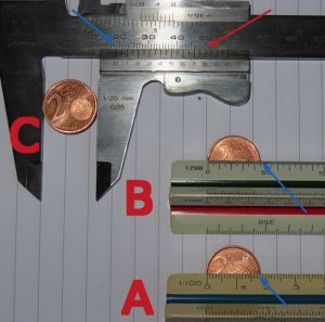
As can be seen in the photo in case A the ruler shows a value of about 18 millimetres (18 marks on the ruler) as shown by the blue arrow, although if we look closely at the photo the zero mark on the ruler does not coincide exactly with the edge of the coin (our hand is not infallible). Moreover, we are not absolutely sure that we are measuring exactly the diameter (we could have measured a little above or below the line that defines the diameter). In other words, apart from the error of the instrument (1 millimetre) there are errors in the measurement itself. That is why it is convenient to make multiple measurements and to make averages, calculate statistical errors, etc. For simplicity we will use the instrument error. So in case A our measurement has an error of 1 millimetre. Now, if we use a more precise ruler, like the one used in case B, we can count 46 marks (see the blue arrow) which would give us 18.4 millimetres with an error of 0.4 millimetres. Finally, with the caliper we see that the diameter is larger than 18 millimetres (blue arrow) but the second scale shows that it is 18.8 millimetres (see red arrow) with a margin of error of 0.1 millimetres. If we were to use a more precise instrument, we could decrease this error to make it, in principle, as small as necessary.
What Heisenberg had discovered went much further, for his relation, written in terms of the standard deviation Δx of the position and momentum Δp, established that for every quantum mechanical system the following inequality had to be satisfied:
$$\Delta x\Delta p\geq\frac{h}{4\pi}$$
That is, if you were able to measure the position of an object with high precision, you would lose precision in the measurement of the momentum (velocity). It was not a question of the instrument to be used, it was a consequence of the quantum theory itself “Only the theory decides what can be observed”: either position or velocity, but both at the same time were impossible to measure with arbitrary precision.

Heisenberg sent a 14-page letter to Pauli on 23 February 1927 telling him what he had discovered and how he had done it, and which served him to write his most famous article (even more so than his first paper on matrix mechanics) “Über den anschaulichen Inhalt der quantentheoretischen Kinematik und Mechanik”, which we mentioned at the beginning of this entry and which he sent for publication just before Bohr’s return. Curiously, when Bohr read it, he discovered an inaccuracy in some of Heisenberg’s comments and insisted that the wave-corpuscle duality should be taken into account, something that Heisenberg resisted. The discussion on this subject was so bitter that at some points Heisenberg burst into tears (there are corroborating witnesses, Pauli among them, who invited him to mediate in the “quarrel” between the Dane and the German).
Heisenberg finally gave in because he realised that Bohr was right and included a final paragraph in his paper, already in print, thanking him.
After the completion of the present work, Bohr’s recent investigations have led to insights which require substantial deepening and refinement of the analysis of the quantum-mechanical relations attempted in this work. In this context, Bohr pointed out that he had overlooked important issues in some of the discussions in this paper. Above all, that observational uncertainty is not exclusively due to the occurrence of discontinuities, but is directly related to the requirement to simultaneously encompass phenomena which have their origin in corpuscular theory on the one hand and in wave theory on the other.
To round off this entry, one of the thought experiments on which Heisenberg based his workings of the uncertainty principle involved an imaginary gamma-ray (high-energy photon) microscope, and it was essential to understand the resolving power of a microscope, something Wein asked him about during his doctoral examination and which Heisenberg did not know how to answer at the time. It is curious how Einstein on the one hand and Wein on the other, both opponents of quantum mechanics, helped Heisenberg in a peculiar way to find what was undoubtedly the most controversial result (and probably still is) of Quantum Mechanics (and probably of all physics) and which ended up destroying the dream of Classical Physics of describing the world with infinite precision. In Heisenberg’s own words
In the strict formulation of the causal law ‘if we know the present we can calculate the future’ it is not the conclusion that fails, but the premise.
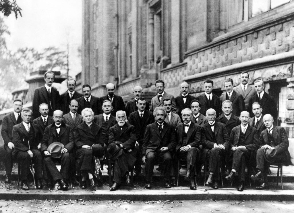
As we have already said, Einstein was not happy with the probabilistic interpretation and much less with the uncertainty principle, so he spent the whole of the 5th Solvay Conference held in 1927, where the leading physicists of the time discussed the recently formulated quantum theory (quantum mechanics, matrix mechanics, the uncertainty principle, among other things) proposing imaginary experiments to Bohr every morning to show him how wrong this interpretation was, experiments that he would dismantle at night. In disgust, Einstein is said to have told Bohr “God doesn’t play dice“, but Bohr, undaunted, replied “Einstein, stop telling God what to do“.
Today quantum mechanics and with it the uncertainty principle are widely accepted, not only because of the enormous success of quantum theory, but also because not a single experiment has been found that contradicts it. We will discuss in a future post this topic and Einstein’s position in the following years.
References
[1] David Lindley, Incertidumbre. Einstein, Heisenberg, Bohr y la lucha por la esencia de la ciencia, Ariel, 2008.
[2] Werner Heisenberg, Diálogos sobre la física atómica. La Editorial Católica. Madrid. 1975. También disponible en la Colección Universal de Círculo de Lectores en el volumen titulado “Física cuántica ( Werner Heisenberg, Niels Bohr, Erwin Schrödinger)” Círculo de Lectores. Barcelona. 1996.
[3] Jagdish Mehra and Helmut Rechenberg, The Historical Development of Quantum Theory, Vol. 6, Part 1: The Completion of Quantum Mechanics 1926–1941, Berlin, Springer, 1982.
On Heisenberg’s life you can read the excellent biography
[4] David Cassidy, Uncertainty: the Life and Science of Werner Heisenberg, New York: W. H. Freeman, 1992.
La referencia del artículo original de Heisenberg traducido al inglés es:
[5] Heisenberg, W. (1927) The Physical Content of Quantum Kinematics and Mechanics. In: Wheeler, J.A. and Zurek, W.H., Eds., Quantum Theory and Measurement, Princeton University Press, Princeton, 62-84.
About the featured image: On the first page of Heisenberg’s letter to Pauli of 23 February 1927 we have superimposed a modified photo of Heisenberg playing dice with Bohr (the original is from the 1936 Copenhagen congress).
Mathematical appendix
A very simple deduction of Heisenberg’s indeterminacy principle from “elementary” physical reasoning can be found in Feynman’s superb lecture.
There are several mathematically rigorous proofs of the uncertainty principle using different mathematical techniques. For mathematical readers we will include here a simplified version of the proof made by Herman Weyl in 1928 (see his monograph The Theory of Groups and Quantum Mechanics, Dover, 1950). As can be seen in this proof, the probabilistic interpretation is an essential premise.
Let us imagine that we have a particle (for example the electron of a hydrogen atom) and we want to know its position and momentum. For simplicity we will consider the one-dimensional case and that our particle is confined to an interval \([a,b]\) (although we could consider the whole real axis we will restrict ourselves to a bounded interval). Let us assume that we know the wave function \(\psi(x)\) that describes a stationary state of our particle, i.e., that it is a solution of the time-independent Schrödinger equation. For simplicity we will also assume that the function \(\psi(x)\) is real. Then, using the Born-Pauli interpretation (discussed above) for the function \(\psi(x)\), the probability of finding the particle in the (infinitesimal) interval \([x,x+dx]\) is \(\psi^2(x)dx\), where \(\int_{a}^b \psi^2(x)dx=1\). Therefore, the mean value \(\overline{x}\) of the position is determined by the integral \(\int_{a}^b x \psi^2(x)dx\) and that of the momentum \(\overline{p}\) (the reader will have to accept that the latter expression, or else refer to any introductory Quantum Mechanics text for a justification of it) is proportional to \(\hbar \int_{a}^b \psi(x)\psi'(x)dx\), where \(\psi’\) denotes the derivative of \(\psi\) and \(\hbar=h/(2\pi)\), being \(h\) the Plank’s constant. Without loss of generality it can be assumed that both \(\overline{x}\) and \(\overline{p}\) are zero. Then the standard deviations (i.e. the uncertainty we would obtain when measuring any of these physical quantities) are, respectively
$$(\Delta x)^2=\int_{a}^b x^2 \psi^2(x)dx\quad \mbox{y}\quad(\Delta p)^2=\hbar^2 \int_{a}^b (\psi’)^2(x)dx.$$
But using the Cauchy-Schwarz inequality that states (for real functions)
$$\left(\int_a^b f(x)g(x)dx\right)^2\leq \int_a^b f^2(x) dx \int_a^b g^2(x)dx,$$
we get
$$(\Delta x)^2(\Delta p)^2 \geq \hbar^2 \left(\int_{a}^b x \psi(x) \psi'(x) dx\right)^2= \hbar^2 I^2.$$
For convenience we will write this last integral \(I\) as the sum of two equal integrals
$$I= \frac12 \int_{a}^b x \psi(x) \psi'(x) dx +\frac12 \int_{a}^b x \psi(x) \psi'(x) dx .$$
Next we will calculate the second integral using integration by parts. For this we will assume that \(\psi(a)=\psi(b)=0\) (this assumption is usual in quantum mechanics, especially in the case of an unbounded interval). Thus, one has
$$\int_{a}^b [x \psi(x)] \psi'(x) dx = x\psi^2(x)\bigg|_a^b-\int_{a}^b [x \psi(x)]’ \psi(x) dx=0-\int_{a}^b \psi^2(x) dx – \int_{a}^b x \psi(x)’ \psi(x) dx$$
which, when substituting it in the expression of \(I\), gives us (remember that \(\int_{a}^b \psi^2(x)dx=1\))
$$I= \int_{a}^b x \psi(x) \psi'(x) dx= – \frac12\int_{a}^b \psi^2(x)dx=-\frac12.$$
Therefore,
$$(\Delta x)^2(\Delta p)^2 \geq \hbar^2 I ^2= \frac{\hbar^2}{4},$$
i.e., we obtain the mathematical expression of the Heisenberg indeterminacy principle \(\Delta x \, \Delta p\geq {\hbar}/{2}\).
Leave a Reply