
As we wrote in a previous post, John Von Neumann (1903-1957) in his article The Mathematician published in 1947, wrote that mathematical ideas originate in the empirical but that once conceived they begin to live a life of their own that can be far removed from the empirical sciences that conceived them. This has undoubtedly been the case of Newton’s and Leibniz’s differential and integral calculus, or the Fourier series of which we spoke here. On this occasion I would like to talk about another of the great mathematical theories that have already lived a long and promising life of their own: the theory of distributions.
A history, even an incomplete one, of the birth of the Theory of Distributions would be too long for a post aimed at a non-specialist audience, so we will take a brief tour of what is probably the most famous distribution of all: Dirac’s \(\delta\) ”function”. The interested reader may consult the superb monograph by J. Lutzen [1] for a detailed discussion.

As Von Neumann did, let’s start by discussing a simple physical problem. Suppose we have a charged sphere whose charge density is defined by the function \(\rho(x,y,z)\) (the reader may think of this as a constant). Then the potential \(\phi(x,y,z)\) associated to the electric field \(\vec{E}\) satisfies Poisson’s equation (in non-dimensional coordinates)
$$
\nabla^2 \phi =\Delta \phi := \frac{\partial^2 \phi}{\partial x^2}+\frac{\partial^2 \phi}{\partial y^2}+\frac{\partial^2 \phi}{\partial z^2}= – \rho.
$$
Knowing the function \(\rho\) we can “easily” find the solution by the formula
$$
\phi(x_1,y_1,z_1)=-\frac{1}{4\pi}\iiint_V \frac{\rho(x_2,y_2,z_2)dV_2}{r_{12}},
$$
where \(r_{12}=\sqrt{(x_1-x_2)^2+(y_1-y_2)^2+(z_1-z_2)^2}\) is the distance between the point \(1\) and the volume element \(dV_2=dx_2\,dy_2\,dz_2\), located at the point \(2\) shown in the figure. The variables \(x_2,y_2,z_2\) run through the whole volume of the sphere \(V\).
The integral runs over the whole sphere. Now imagine that we have a given charge \(q=1\) contained in the sphere and we make \(r\), the radius of the sphere, tend to zero, what do we find? It is obvious that there is a problem since the charge density is the value of the charge divided by the volume of the sphere, but the volume of the sphere tends to zero and, therefore, the density tends to infinity, how can we solve this dilemma? On the other hand, it is clear that if \(r\to0\) what we have is the interaction of two punctual charges and, therefore,
$$
\phi(x_1,y_1,z_1)=-\frac{1}{4\pi r_{01}},
$$
where \(r_{01}\) is the distance between the centre of the sphere and the point \(1\). That is to say, we have on the one hand that \(\rho(x_2,y_2,z_2)\) is zero at every point except at the centre \((x_0,y_0,z_0)\) of the sphere, but at this centre \(\rho\) tends to infinity. Let us call the resulting function \(\delta(x_2,y_2,z_2)\). That is, we have something like
$$
(1)\qquad \qquad \delta(x,y,x)=
\begin{cases}
0, & \mbox{ if } (x,y,z) \neq (x_0,y_0,z_0), \\[3mm]
\infty, & \mbox{ if } (x,y,z) = (x_0,y_0,z_0).
\end{cases}
$$
Which does not make much sense from a mathematical point of view. But from the above it also follows, at least formally, that
$$
\phi(x_1,y_1,z_1)=-\iiint_V \frac{1}{4\pi}\frac{\delta(x_2,y_2,z_2)}{r_{12}}dx_2dy_2dz_2=-\frac{1}{4\pi r_{01}}.
$$
Besides, in his acclaimed memoir Théorie analytique de la chaleur, Fourier encounters a similar problem. During the study of the heat equation, Fourier proves (in his own very unrigorous way) the following expression (page 260)
$$
f(x)=\frac1\pi \int_{-\pi}^{\pi}\left\{ \frac12 + \sum_{k=1}^{\infty} \cos k(x-y) \right\}f(y)dy,
$$
and then assert that
The expression \(\frac12 + \sum_{k=1}^{\infty} \cos k(x-y)\) represents a function of \(x\) and \(y\) such that if it is multiplied by any function \(f(y)\) and integrated with respect to \(y\) between the bounds \(y=-\pi\) and \(y=\pi\), the proposed function \(f(y)\) becomes the similar function of \(x\) [i.e., \(f(x)\)] multiplied by the semicircle \(\pi\).
If we take a look at the function \(d(x,y)=\frac12 + \sum_{k=1}^{\infty} \cos k(x-y)\), we can discover an interesting property. If \(x=y\) the sums \(\frac12 + \sum_{k=1}^{N} \cos k(x-y)=N+\frac{1}{2}\) which tends to infinity if \(N\to\infty\), and if \(x-y\) is somewhat away from zero the value is quite a bit smaller. Graphically, for \(N=1000\), we see it in the following figure:
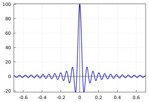
In other words, it is very similar to the \(\delta\) function defined above, but in this case in a single variable. Specifically
$$
\lim_{N\to\infty} \frac1{2\pi}\left(1 + \sum_{k=1}^{N} \cos k(x-y)\right) = \delta(x-y)=
\begin{cases}
0, & \mbox{ if } x \neq y, \\[3mm]
\infty, & \mbox{ if } x=y.
\end{cases}
$$
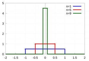
Let’s continue with another example in one variable. In this case let’s take a string held by its ends to which a force is applied concentrated on a small piece of the string, for example at the point \(x=0\) and whose expression is (see the figure)
 $$
$$
f_n(x)=\left\{\begin{array}{ll} \dfrac{n}2, & |x|\leq \dfrac1n, \\[3mm] 0, & |x|>\dfrac1n,
\end{array}\right.
$$
If we take the limit when \(n\to\infty\) of \(f_n(x)\) we have again something similar to (1)
$$
\lim_{n\to\infty} f_n(x)=\delta(x)=
\begin{cases}
0, & \mbox{ if } x \neq 0, \\[3mm]
\infty, & \mbox{ if } x =0.
\end{cases}
$$
Let’s choose now any continuous function \(\phi(x)\) and then calculate the following integral
$$
\int_{\mathbb{R}} \phi(x) f_n(x)dx=\frac n2\int_{-1/n}^{1/n} \phi(x)dx=\phi(\xi_n),
$$
where \(\xi_n\in(-1/n,1/n)\). For the last equality the mean integral theorem has been used. Since \(\phi(x)\) is continuous, if we take the limit when \(n\to\infty\), we have that \(\lim_{n\to\infty}\xi_n=0\), and therefore \(\lim_{n\to\infty}\phi(\xi_n)=\phi(0)\).
This last approximation was very common in physics. One of the first to formalise it was Paul M. Dirac. In his book Principles of Quantum Mechanics (5th Ed. page 58) [2] he introduces the function \(\delta\)
$$
\begin{cases}
\delta(x)=0 & \mbox{if } x\neq 0, \\[5mm]
\displaystyle\int_{\mathbb{R}} \delta(x) dx=1.&
\end{cases}
$$
and explains
To get a picture of \(\delta(x)\), take a function of the real variable \(x\) which vanishes everywhere except inside a small domain, of length \(\epsilon\) say, surrounding the origin \(x = 0\), and which is so large inside this domain that its integral over this domain is unity. The exact shape of the function inside this domain does not matter, provided there are no unnecessarily wild variations […] Then in the limit \(\epsilon\to 0\), this function will go over into \(\delta(x)\).
\(\delta(x)\) is not a function of \(x\) according to the usual mathematical definition of a function, which requires a function to have a definite value for each point in its domain, but is something more general, which we may call an ‘improper function’ to show up its difference from a function defined by the usual definition. Thus \(\delta(x)\) is not a quantity which can be generally used in mathematical analysis like an ordinary function, but its use must be confined to certain simple types of expression for which it is obvious that no inconsistency can arise. The most important property of \(\delta(x)\) is exemplified by the following equation, \(\int_{\mathbb{R}} \delta(x) \phi(x)dx=\phi(0)\), where \(f(x)\) is any continuous function of \(x\).
Dirac himself lists a large number of properties of the function \(\delta(x)\) and brings back the definition of the \(\delta(x)\) introduced by Heaviside in 1899: \(\delta(x)\) is the derivative of the Heaviside step function \(h(x)=0\) if \(x<0\) and \(h(x)=1\) if \(x\geq1\). As Lutzen says in his book [1], Dirac must have been familiar with Heaviside’s operational calculus since Dirac studied electrical engineering, and this was one of the typical mathematical tools.
At this point it is a good time to explain how to define the \(\delta(x)\) function in a mathematically rigorous way. The answer is ”The theory of distributions” developed by Laurent Schwartz. And this is where the mathematics takes on a life of its own again.

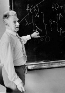
Let us begin with a brief profile of its discoverer: Laurent Schwartz was born in 1915 into a non-practising Jewish family. His father was the first Jewish surgeon in the hospitals of Paris and his mother was passionate about nature, something she passed on to her three children. At school he excelled especially in Latin, literature and mathematics, but fortunately for everyone he eventually opted for mathematics. He studied at the famous École Normale Supérieure (ENS), graduating in 1937. During his time at the ENS he was attracted to communist ideas, but the Stalinist purges of 1936 turned him into a militant Trotskyist, until 1947 when he left Trotskyism disappointed. After that he remained a lifelong advocate of human rights. In 1940 he moved with his wife to Clermont-Ferrand and began to frequent the famous circle of self-declared Bourbaki mathematicians, which he joined as a full member in 1942. In 1942 he defended his doctoral thesis and had to go into hiding in a small village to escape the persecution of Jews in Nazi-occupied France until August 1944. After a brief stay in Grenoble, he moved to the Faculty of Science in Nancy, where he spent seven years and where he developed the theory of distributions. In 1950 he received the Fields Medal for his theory of distributions, shortly before his now classic monograph Théorie des Distributions was published. In 1952 he moved to Paris where he taught at the Sorbonne and the École Polytechnique. Among his many students were great mathematicians such as A. Grothendieck and J.L. Lions. Schwartz died on 4 June 2002 at the age of 87.
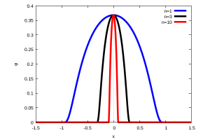
The basis for understanding the theory of distributions is to define the space of test functions \(\mathcal{D}(\mathbb{R})\) (nowadays called Schwartz space). This is the set of infinitely differentiable functions, that is, having derivatives of any order and compact support, i.e., which are only different from zero in the interior of a set \([a,b]\subset\mathbb{R}\). An example of such test functions are the functions
$$
\varphi_n(x)=\left\{\begin{array}{ll} \exp\left(-\dfrac1{1-n^2x^2}\right), & |nx|<1, \\[3mm] 0, & |nx|\geq1.
\end{array}\right.
$$
which we can see in the figure for \(n=1,3,10\):
Using this space Schwartz defined a \(T\) distribution as an application \(T:\mathcal{D}(\mathbb{R})\mapsto\mathbb{C}\) which is linear and continuous. Although this concept is in general complicated, it can be thought of as a linear function whose variables are the \(\varphi(x)\) functions of the space. One of the simplest examples, of course, is the Dirac \(\delta\) function (so named by Schwartz in honour of Paul M. Dirac). Thus, the Dirac delta \(\delta(x)\) is the distribution defined by
$$
\delta:\mathcal{D}(\mathbb{R})\mapsto\mathbb{C},\quad \delta(\varphi)=\varphi(0).
$$
Interestingly, such a simple definition gave mathematical rigour to a huge number of physics and engineering problems such as those discussed above. In fact, two of the most commonly used are the following distributions
$$
\lim_{L\to\infty } \dfrac{1}{\pi} \dfrac{\sin(Lx)}{x}=\delta(x), \quad \mbox{y}\quad
\dfrac{1}{2\pi} \int_{-\infty}^{\infty} e^{i k x}dx =\delta(k).
$$
The latter appears in many books on quantum mechanics and quantum field theory. Schwartz himself wrote a book on this subject entitled Application of Distributions to the Theory of Elementary Particles in Quantum Mechanics based on lectures he gave at the National University of Argentina, in Buenos Aires and at Berkeley.
It must be said in all fairness that ideas very similar to Schwartz’s were used by the Soviet mathematician Sergei L. Sobolev in 1935-1936, on works unknown to Schwartz probably due to the time and the years of their publication in Stalin’s Soviet Union. Sobolev was born in St. Petersburg in 1908. His father was a lawyer and his mother a professor of literature and a doctor. He studied mathematics at the University of Leningrad (now St. Petersburg) and graduated in 1929. He worked first at the Leningrad Seismological Institute and then from 1934 at the Steklov Institute of Mathematics. He devoted himself mainly to the study of partial differential equations, and in particular to the Cauchy problem of hyperbolic equations with variable coefficients. To this end, he introduced techniques very similar to those of Schwartz, including the generalised derivative and a whole class of functions now called Sobolev spaces in his honour. Sobolev devoted part of his research in the 1940s to the war effort during the Second World War. In particular, he was involved in the Soviet atomic bomb project, leading and supervising several teams specialising in the computational calculations for the bomb project between 1942 and 1949. For this work, in January 1952, Sobolev received the highest title awarded in the USSR: he was declared a Hero of Socialist Labour for outstanding service to the state (he had previously received two Stalin prizes).
If Sobolev introduced the necessary tools, some of them very similar to Schwartz’s, to solve a very specific problem: the so-called Cauchy problem, Schwartz developed a very versatile theory capable of solving countless problems. In Lutzen’s words
Sobolev invented distributions, but it was Schwartz who created the theory of distributions.
Para saber más:
[1] J. Lutzen, The prehistory of the theory of distributions. (Studies in the History of Mathematics and Physical Sciences, Vol. 7) Springer (1982)
[2] P.A.M. Dirac, The Principles of Quantum Mechanics, Oxford University Press, 1th Ed. 1930, 4th Ed. 1958.
[3] S.S. Kutateladze, Sobolev and Schwartz: Two Fates and Two Fames, arXiv:0802.0533 [math.HO]
[4] F. Bombal, Laurent Schwartz, el matemático que quería cambiar el mundo, Volumen 6, número 1 (2003).
Leave a Reply