Frank Plumpton Ramsey died at the age of 26 but led a very active life. He excelled in at least three fields Philosophy, Mathematics and Economics. In mathematics he is known for Ramsey’s theorem which was first just a lemma in a paper on mathematical logic and which is the beginning of what is now called Ramsey Theory.
Ramsey’s theorem refers to graphs, a graph is a set of vertices \(V\) and a set of edges \(A\) each joining two vertices. The complete graph is a graph with \(n\) vertices and an edge between every two vertices. The complete graph with \(n\) vertices is denoted by \(K_n\). In graph theory it is common to consider colorings of the vertices. But we will only talk about colorings of the edges of the complete graph \(K_n\). Coloring the complete graph with two colors is equivalent to separating the edges into two classes, which we will always call red and blue. Given a vertex \(x\) we define its neighborhoods \(N_B(x)\) the set of vertices \(y\) such that the edge \(xy\) is blue, and \(N_R(x)\) the set of vertices that form a red edge with \(x\). Naturally we will always have that \(N_R(x)\cup N_B(x)\) is the set of all vertices minus \(\{x\}\). We will use \(|X|\) to denote the cardinal of a finite set and \(e_R(X,Y)\) to denote the number of red edges joining the sets \(X\) and \(Y\).
Ramsey’s theorem states that if we have two numbers \(k\) and \(\ell\) there exists a number \(R=R(k,\ell)\) such that in any coloring of the complete graph of \(n\ge R\) vertices we have either \(k\) vertices with all the edges joining them red, or there exist \(\ell\) vertices in which all the edges are blue. That is, the graph contains either a complete \(K_k\) all-red graph or a \(K_\ell\) all-blue graph. The numbers \(R(k,\ell)\) are called Ramsey numbers.
The philosophy of Ramsey’s theory is summarized in the motto: there will always be some order in any sufficiently large disorder, or more poetically: we will find life in any sufficiently large universe.
Today’s entry is about efforts to estimate the size of the numbers \(R(k,\ell)\) and in particular of the diagonal Ramsey numbers \(R(k)=R(k,k)\). What we know of the exact value of these numbers is collected in the table below taken from Lane Barton IV.
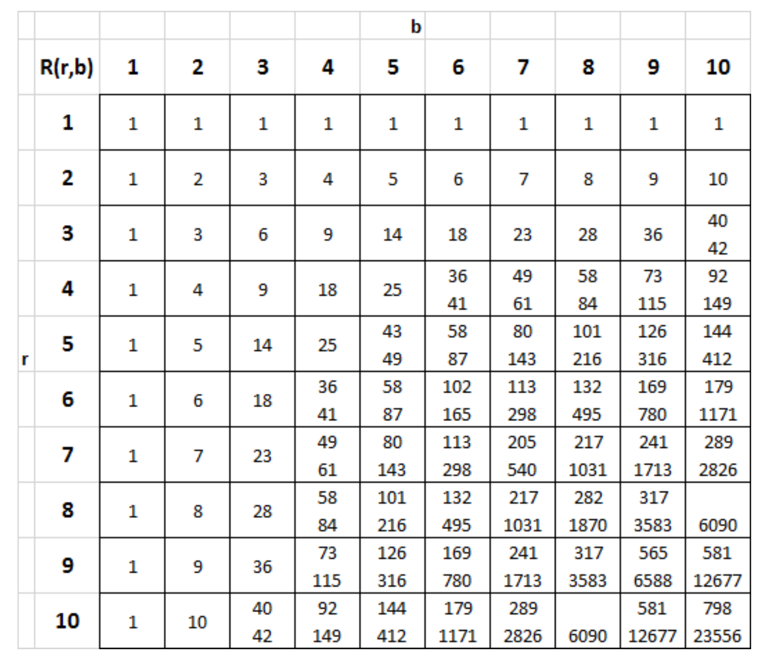
When there are two numbers, it means we only know the range, e.g., \(102\le R(5,5)\le 165\).
Progress
In 1928, Ramsey proved that the Ramsey numbers \(R(k,\ell)\) are finite. A little later Erdös and Szekeres proved that $$R(k)\le 4^k.$$ They actually proved the inequality $$R(k,\ell)\le \binom{k+\ell}{\ell}.$$ Erdös asked whether Ramsey numbers would really be so large. So in 1947 Erdös returned to the subject, and succeeded in proving a lower bound. His paper had two fundamental ideas, which have been applied later in numerous problems. The Probabilistic Method and Random Graphs. We can find entire books devoted to each of these two ideas of Erdös.
The probabilistic method consists of proving the existence of an object with certain characteristics, considering it as an element of a probability space and then proving that the probability of the objects with those sought characteristics is positive (and often close to \(1\)). Random graphs consist of constructing a graph with \(n\) vertices by randomly assigning a probability to each of the possible \(\binom{n}{2}\) edges. In our problem we can color the edges of the complete \(K_n\) graph using red or blue depending on the result of a coin flip.
Erdös proves that the probability of finding a monochromatic \(K_k\) by randomly coloring the edges of \(K_n\) being \(n=2^{k/2}\) is strictly less than \(1\). So there must exist colorings for which \(K_k\) monochromatic does not exist. That is \(R(k)>2^{k/2}\).
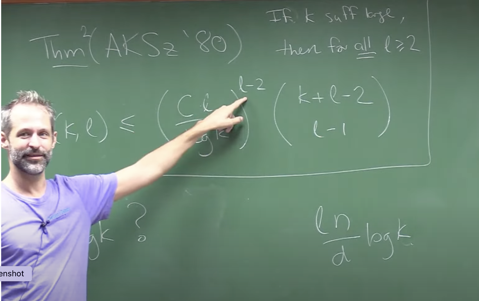
After Erdös’ work in 1947, we had the inequalities $$2^{k/2}\le R(k)\le 4^k,\quad R(k,\ell)\le \binom{k+\ell}{\ell}.$$ Subsequent progress has been slow and very modest. Thomason (1988), Conlon (2009) and Sah (2023) get $$R(k)\le 4^{k-c(\log k)^2},\quad R(k,\ell)\le e^{-c(\log k)^2} \binom{k+\ell}{\ell}.$$
The preprint we are discussing today that appeared in March (of 2023) in arXiv, manage to prove that $$R(k)\le (4-2^{-7})^k,\quad R(k,\ell)\le e^{-\ell/50+o(k)}\binom{k+\ell}{\ell}.$$ The work, which breaks an 86-year-old barrier, is a joint effort of Robert Morris and Marcelo Campos, professor and PhD student at IMPA, Simon Griffiths of the Pontifical University of Rio de Janeiro and Julian Sahasrabudhe of Cambridge.

The original source: Erdös-Szekeres’ argument
The work we discuss uses a very different technique than the last works on the subject that used the idea of quasi-random graphs. They use a more direct method and its closest antecedent is the proof of the \(R(k)\le 4^k\) inequality of Erdös and Szekeres. We will first explain this proof in the form in which it is presented by Robert Morris in his Ph.D. course that we cited in the last section. In this way the proof of \(R(k)\le 4^k\) is very transparent and I think we can all enjoy it. Moreover, this will give us an idea of the style of the Campos-Morris-Griffiths-Sahasrabudhe proof.
We can describe its proof by means of an algorithm. We will have two sets of vertices \(A\) and \(B\) and another set \(X\) evolving in the algorithm. Starting with \(A=B=\emptyset\) and \(X\) the complete set of vertices.
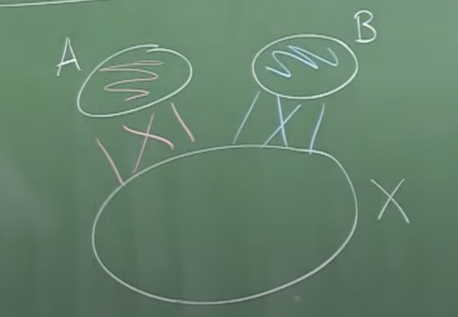
In the end we intend to obtain in \(A\) a complete red graph and in \(B\) a blue one and if \(|X|\) is sufficiently large one of the two will have at least \(k\) points. At each stage of the algorithm we will add a point to either \(A\) or \(B\) and our set \(X\) will be divided by \(2\). The algorithm runs as long as \(X\) is not empty.
In each step of the algorithm we choose a point \(x\in X\) and we will pass it to \(A\) or \(B\). If \(|X\cap N_R(x)|\ge |X|/2\) we will put $$A\to A\cup\{x\}, \quad X\to N_R(x)\cap X,\quad B\to B.$$ if on the contrary \(|X\cap N_B(x)|\ge |X|/2\) then we will put $$B=B\cup\{x\}, \quad X\to N_B(x)\cap X,\quad A\to A.$$ Since \(N_B(x)\cup N_R(x)=X\) one of the two alternatives are satisfied. At each step \(A\) or \(B\) grows. Notice that the edge color conditions between \(A\), \(B\) and \(X\) hold at each step.
At each step the set \(X\) decreases but at least half of its vertices remain, so that at each step we will have \(|X|\ge 2^{-|A|-|B|}n\) where \(n\) is the total number of vertices. We can continue the algorithm as long as \(X\) is not empty. Then in the end we will have \(|A|+|B|\ge 2k\) if we assume that \(n\ge4^k\). In that case one of the two \(A\) or \(B\) will be greater than \(k\) and we will have found a complete single color graph with at least \(k\) vertices.
Actually Erdös and Szekeres prove something else. First we must define \(R(k,\ell)\), as the minimum \(n\) such that any coloring of \(K_n\) contains either a complete red copy of \(K_k\) or a complete blue copy of \(K_\ell\). Then they prove $$R(k,\ell)\le \binom{k+\ell}{\ell}.$$ We can prove this essentially with the same proof but separating the blue or red steps in the algorithm according to whether \(|N_R(x)\cap X|\ge \frac{k}{k+\ell}\) or \(|N_B(x)\cap X|\ge \frac{\ell}{k+\ell}\).
The book’s idea
The next idea we should handle comes at least from Thomason: Let us try to find a large monochromatic “book”. Books seem to have a place in many parts of combinatorics and it is difficult to know their origin. We will work with red books.
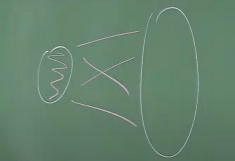
The spine is the set of vertices on the left. All the edges between vertices of the spine are red and all the edges between the spine and the set on the right are red. Each point in that set on the right can be thought of as a leaf. If we think about it this kind of sets have already appeared in the Erdös-Szekeres proof.
If the number of leaves is greater or equal than \(R(k,k-t)\) and the spine has cardinal \(t\) we will obtain a blue \(K_k\) or a red \(K_{k-t}\). [notice that \(R(k,\ell)=R(\ell,k)\)] as in the figure.
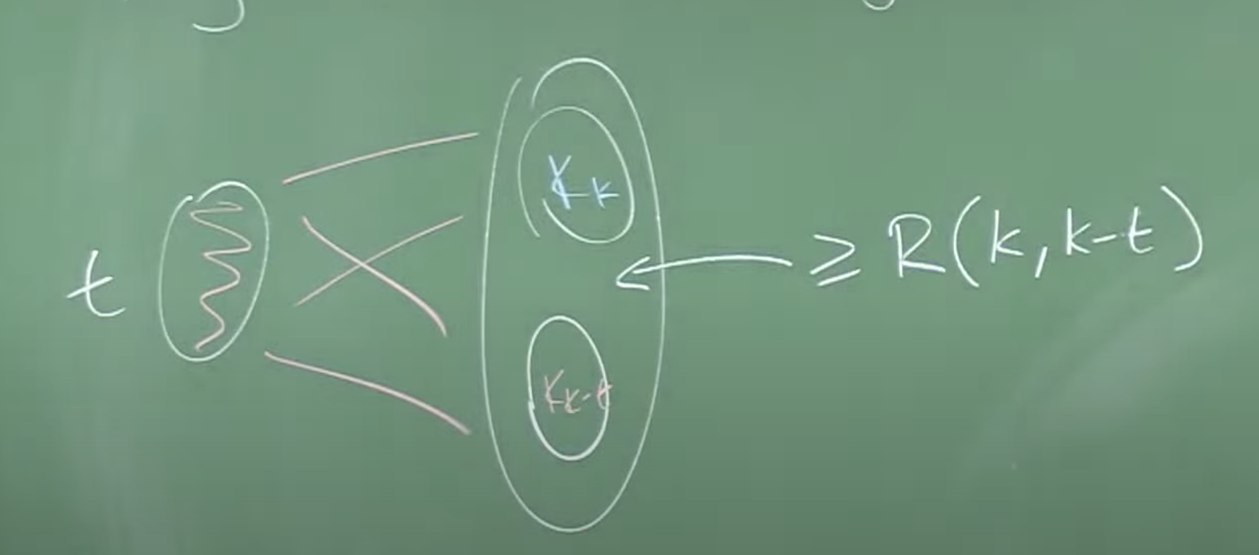
This would finish our work as we would have either a blue \(K_k\) between the leaves, or a red \(K_k\) joining the spine with the copy of \(K_{k-t}\) on the leaves. But we must do this quantitatively to get \(R(k)\) bounded.
There is a conjecture by Thomason that you can find a single-color book with \(t\)-spine and \(2^{-t} n\), pages. This conjecture would imply our result.
The algorithm of Campos, Griffiths, Morris and Sahasrabudhe
As we say we modify the Erdös-Szekeres proof. We start from a coloring of \(K_n\) which we assume contains neither a red \(K_k\) nor a blue \(K_\ell\). We don’t look for a blue book. We will only look for the red one. We will now have two sets \(A\) and \($ that start out empty and two other disjoint sets \)latex X$ and \(Y\), related as in the figure
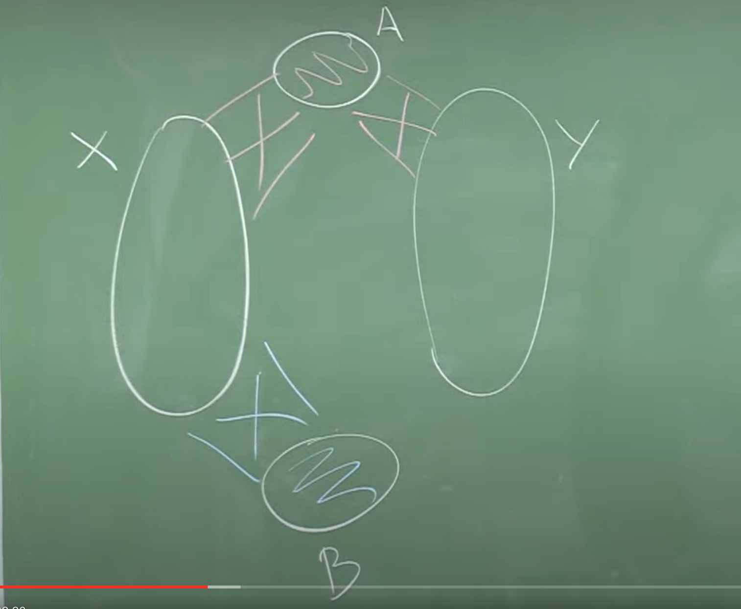
The final book has spine \(A\) and the set of leaves will be \(Y\). The algorithm is a succession of steps, but now there are four types of steps:
(a) Red Steps: When we have a point \(x\in X\) with many red neighbours in \(X\) and in \(Y\), we will add it to \(A\) $$A\to A\cup\{x\},\quad X\to N_R(x)\cap X,\quad Y\to N_R(x)\cap Y, \quad B\to B.$$ We also need to guarantee that the density of red vertices between \(X\) and \(Y\): \(p:=\frac{e_R(X,Y)}{|X|\cdot|Y|}\) does not decrease much in this step.
(b) Big Blue steps: If we cannot make a red step, possibly it is because the points \(x\in X\) have \(N_R(x)\cap X\) small, in that case there are many blue edges in \(X\) and we can find a book \((S,T)\) inside \(X\) and in that case we make the change $$A\to A, \quad B\to B\cup S,\quad X\to T,\quad Y\to Y.$$ This movement maintains our color requirements, but generally decreases the value of the density \(p\), this forces us to previously make a step of regularizing \(X\).
(c) Degree regularisation: We remove from \(X\) the points with intersection \(N_R(x)\cap Y\) small $$X\to\{x\in X\colon |N_R(x)\cap Y|\ge (p-\varepsilon^{-1/2}\alpha)|Y|\}.$$ But we will not try to explain the parameters in this election.
(d) Density-boost step: When there are few points in \(X\) with many blue edges in \(X\) or else any red step decreases \(p\) too much, we increase this density by choosing a point \(x\) with few blue edges and setting $$A\to A,\quad B\to B\cup \{x\},\quad X\to N_B(x)\cap X,\quad Y\to N_R(x)\cap Y.$$
In a first attempt to obtain \(K_k\) with this algorithm, we would like to find a book \((A,Y)\) with $$|Y|\ge \binom{2k-t}{k-t}\ge R(k,k-t),\quad |A|=t.$$ But this along with the Erdös-Szekeres bound for \(R(k,\ell)\) is almost, but not quite enough. That is when they had the idea to apply the method to improve the Erdös-Szekeres bound for \(\ell\) relatively smaller than \(k\). Thus the algorithm allows them to prove $$R(k,\ell)\le e^{-\ell/50+o(k)}\binom{k+\ell}{\ell}.$$ With this bound in hand it is possible to apply the algorithm again and achieve the goal.
Some answers to my question to the authors
J.: I am curious about how four mathematicians start to think about such a seemingly difficult problem. I imagine that at the time you had an idea for attacking the problem that must not have been very precise. Can you explain that moment?
The project began during the last few weeks of Julian’s postdoc at IMPA. We are always on the lookout for interesting and difficult problems to work on, and we had recently learnt (from a paper of David Conlon) about an old conjecture of Thomason on the Ramsey numbers of “books” which, if true, would imply an exponential improvement on the diagonal Ramsey numbers. Our usual strategy is to spend a few days discussing a new problem in front of the board, coming up with ideas and trying to understand the main obstructions, and then decide whether we have an approach that’s worth pursuing further. In this case we very quickly came up with a strategy which looked extremely promising, and reduced the problem to a conjecture about “asymmetric” subsets of high-dimensional spheres, which looked like it should be do-able. From that moment we were hooked.
J.: I was quickly watching the first video of Robert Morris’s PhD course, something said about a 5-year proof hiatus, until the idea comes up. I think this a useful information for the students in Sevilla, could you give more details, did you have a preprint or something stopped while, was the equip the same during all that time?
During the following five years we threw everything we had at our spheres conjecture, to no avail. We tried all kinds of different techniques – algebraic, analytic, probabilistic, geometric, combinatorial – but nothing seemed to work. We would meet at IMPA each (Brazilian) summer to work on the problem, and in both 2020 and 2022 we thought we were close to a solution, but both times the proof collapsed on closer inspection. We were disheartened, and close to giving up, but late last year we agreed to have one final try.
The breakthrough occurred almost immediately when we arrived in Rio at the start of January. The key idea was to give up on our spheres conjecture, and instead try to bound the Ramsey numbers in the easier “off-diagonal” setting. From that simple sideways step, everything suddenly moved extremely quickly: within a week or so we had a simple (and purely combinatorial) proof far from the diagonal, and within another couple of weeks we discovered that, miraculously, the method could be pushed *just* far enough to reach the diagonal. Every obstruction we met was quickly dealt with using some idea or other that we had come up with years earlier, and by early February we had a draft of the proof written down.
To learn more
So far it has had relatively little impact on the network. We have a presentation in Nature, an announcement on the web, an entry in
Live-Science. Also there is an announcement in NewScientist but not free.
The best explanation of the work is the one given by one of the authors Robert Morris in a Ph.D. course at IMPA. The Institute of Pure and Applied Mathematics in Rio de Janeiro.
Or, of course, the preprint in arXiv:
Marcelo Campos, Simon Griffiths, Robert Morris y Julian Sahasrabuhde, An exponential improvement for diagonal Ramsey, arXiv:2303.09521. (16 de marzo de 2023).
On the general subject of Ramsey’s numbers there is a paper published in the Dutch magazine Nieuw Archief voor Wiskunde, explaining what we saw in our entry The happy end problem:
Ross J. Kang, Parties a smidgen smaller, Nieuw Archief voor Wiskunde, 21} (2020) 232-235. (be careful, downloads the pdf).
We have used the table in the publication:
Lane Barton IV, Ramsey Theory 23 páginas (2016). (be careful, downloads the pdf).
Ramsey was a really interesting character. An article in the New Yorker explained some of the character The man who thought too fast. There are two relatively recent biographies:
Cheryl Misak, Frank Ramsey, a sheer excess of powers, Oxford University Press, 2020.
Karl Sabbagh, Shooting Star The brief and brilliant life of Frank Ramsey.
and a paper in Mathematical Intelligencer:

It is probably not a good idea to cite a paper about “Sir Woodsor Kneading” that at the end states, “As the reader has likely suspected, the first section is correct but the rest of the story is a hoax.”
Thank you for the warning. I’m sorry I let myself get fooled like that. I have deleted the small paragraph, it adds nothing to the post. That renders your comment meaningless, but what I can’t do is keep the mistake. I appreciate you letting me know so I can correct it.